Earlier this year the UK had a General Election, which, in many quarters, was declared a landslide victory for Labour. Certainly we have – thank goodness – a new government, and the switch towards Labour in terms of the number of seats (and hence MPs) was dramatic. But there remains an ongoing debate as to what extent the result was driven by Labour positively winning the election or whether it was more that the demonstrated incompetence of the previous government, the Conservatives, meant that any other “big party” was almost guaranteed to win.
There are also some questions around the “fairness” of the result in terms of the first-past-the-post system our country which translates number of votes into number of seats which is the main determination of which party gets to form the government, i.e. who “won”. So I wanted to see real numbers on this. Surely it shouldn’t be difficult to see how many and what proportion of votes each party got and compare it to their performance in past elections. Is it truly the case that Labour “lucked out” and got an unusually high number of seats vs their vote count, or is this just a standard British idiosyncrasy that happens every few elections? It’s not as if our electoral system fundamentally changed in recent times and there’s no serious accusation of electoral fraud (we’re not the US after all!). But I would like to understand the numbers and whether we saw an aberration that might trouble us in principle – even if I personally am reasonably pleased about the outcome.
As it transpires, I couldn’t quickly find a big table of nicely granular formatted-for-analysis UK general election results from the distant past right up to 2024. Plenty of articles out there compare the 2024 results to the 2019 results, but I was more interested in the longer-term trends. I suppose no-one had data teams back in 1950, or at least not ones that would upload their output to the nowhere-near-yet-existing internet. So what’s an analyst to do apart from accidentally enter the wormhole of constructing such a dataset? So that’s what I ended up doing.
The data
If you just want to see the data – roughly one row per constituency per party standing in it per election from 1918 through to 2024 – then it’s here on Github or here on Data.world. Below I’ll go into more of exactly what it is, where it’s from, and its (extensive) limitations.
The columns I provided in this version are as follows:
| Field | Description |
|---|---|
| election | Which year’s election this data is for. |
| id | An ID used by the datasource to refer to a constituency per election – not present for all elections. |
| ons_id | Another ID used by the datasource to refer to a constituency per election – not present for all elections. |
| constituency | Name of the constituency that the votes were cast in. |
| country_region | Region of the country the constituency is in. |
| country | Which country the constituency is in – not present for all records. |
| electorate | The size of the electorate within the constituency. |
| total_votes | How many valid votes were cast in total – all parties combined – within this constituency. |
| party | Which party this row refers to. |
| votes | How many votes were cast in this constituency for this party. |
| share_of_vote | The % of valid votes that were cast in this constituency were for this party. |
The sources
I first considered scraping tables Wikipedia’s collection of UK general election pages to get the numbers, but in practice they aren’t all formatted the same way and it seemed like it might end up being a lot of work. In the end I took data published by the House of Commons Library, which also has the bonus of seeming as official as anything could be.
After a bit of searching I actually thought some kind civil servant had already made what I wanted! See the excitingly named “General election results from 1918 to 2019” which has an accompanying CSV and (more details) Excel file. It indeed was the Excel file that I ended up using. But, as so often with the data published by our Government, it’s published in a format that might be a somewhat accessible to readers but a bit less useful for data nerds who want to do their own analysis.
I can’t complain too much. The UK state has a decent amount of data available for download, and some interesting sounding data teams. We’ve at least moved on from the days when it was all in PDFs to a world of Excel and CSV. But still, if I wanted to compare election results over time then I was going to want tidy data. Not the set of data that arrived, which was a set of 28 Excel sheets having occasionally inconsistent column names and positions, along with a load of analytically-incompatible cruft added in semi-random places in the name of formatting and notes.
You can download and check the code I wrote to do this here if you like. My aim was to, as painlessly as possible, transform nice colourful wide data that looked like 28 sheets of this:

Into less attractive but much more easily analysable long data that looked like this:

Coding the clean-up
I wanted to clean up and combine the data into a single, reasonably consistent, datafile. To do this I used R. Some parts of the code are presented below, or you can review the full script on Github here.
If you want to reproduce it, then the libraries I used during this effort were as follows:
library(tidyverse)
library(readxl)
library(tidyverse)
library(janitor)
library(scales)
library(assertr)
I started by retrieving the name of all worksheets in the 1918-2019 results Excel workbook, using the readxl library.
library(readxl)
historic_sheet_names <- excel_sheets(historic_results_file)
I could then use those names to loop through each sheet of the workbook to download and clean the data it contained, before combining them all at the end.
for (sheet in historic_sheet_names)
{
  # Get the contents of the current sheet
  election_results <- read_excel(historic_results_file, sheet = sheet, skip = 1)

  # Initialise a variable we can manipulate to get a clean dataset to match the data we just read in
  # (not strictly necessary but it also does no harm - might make debugging any problems easier)

  election_results_clean <- election_results

  # Use the first row as column names, where a value exists

  election_results_clean <- row_to_names(election_results, row_number = 1, remove_row = TRUE) |>
    clean_names()

  # remove cols that are all NA

  election_results_clean <- election_results_clean |>
    select_if(~ !all(is.na(.)))

  # Remove cols where the first value is vote share.
  # We can calculate this from the rest of the data if we need it later

  election_results_clean <- election_results_clean[, !unlist(election_results_clean[1, ]) %in% c("Vote share", "Votes Share")]

  # Now if the name of the field is "na" starts with na_ we rename it to the value in the first row.
  # We can't just look for "starts with na" because sometimes legitimate party names start with those letters.

  # Loop through the columns
  for (i in seq_along(election_results_clean)) {
    # Check if the column name starts with "na_" or is exactly "na"
    if (startsWith(colnames(election_results_clean)[i], "na_") | colnames(election_results_clean)[i] == "na") {
      # Set the column name to the first value in the column
      colnames(election_results_clean)[i] <- election_results_clean[1, i]
    }
  }

  # Ensure the column names are 'safe' per R's rules

  election_results_clean <- clean_names(election_results_clean)

  # Remove first row now we extracted it into our column names

  election_results_clean <- election_results_clean[-1, ]

  # Remove any rows with no constituency name. These are usually blank rows or interpretation notes

  election_results_clean <- filter(election_results_clean, !is.na(constituency))

  # Any column names that at this stage still start with "na_" or are exactly "na" are random notes or other such data we'll not keep in our dataset

  election_results_clean <- select(election_results_clean, -starts_with("na_"), -any_of(c("na")))

  # Now we pivot it to a long version where the per-party results are transformed from columns into rows
  # And we move any rows with null votes - these will be constituencies where the relevant party didn't field a candidate.

 # Some sheets contain different field names to other in terms of the columns that don't relate to a party. We'll drop those, but note that not all sheets contain all fields so we use "any_of" to avoid column not found errors.


  election_results_clean_long <- election_results_clean |>
    pivot_longer(
      cols = -any_of(c("id", "constituency", "county", "country", "country_region", "seats", "electorate", "total_votes", "turnout", "ons_id")), # this are the columns that don't relate to party - not all of them appear in each year's sheet
      names_to = "party",
      values_to = "votes"
    ) |>
    filter(!is.na(votes))

  # Add a field to keep track of which election these results are from. This is based on the sheet name we read in.

  election_results_clean_long <- election_results_clean_long |>
    mutate(election = sheet)

  # Now we can append our long, clean results from this sheet to the final dataset

  historic_election_results <- bind_rows(
    historic_election_results,
    election_results_clean_long
  )
}
Then, moving on to the 2024 data, I found a spreadsheet from the same source. Of course it, once again, had different column names and data values than the 1918-2019 file. Aargh.
So I imported its contents and did some renaming and rejigging to get it into the same sort of long format as the above code did for the earlier file.
# The columns are named differently to the dataframe that we've been constructing so far, and there are more of them.
# Rename and preserve only the columns in common
# Constituencies were in capital letters in the historic file. Transform these similarly.

election_results_2024 <- election_results_2024 |>
  select(ons_id,
    constituency = constituency_name,
    country_region = region_name,
    country = country_name,
    electorate,
    total_votes = valid_votes,
    con:all_other_candidates
  ) |>
  mutate(
    election = "2024",
    constituency = toupper(constituency)
  )

# Now we need to convert the 2024 results to a similar style long table as we have with the historic results

election_results_2024_long <- election_results_2024 |>
  pivot_longer(
    cols = (con:all_other_candidates),
    names_to = "party",
    values_to = "votes"
  ) |>
  filter(!is.na(votes))
The 2024 file also unkindly refers to the parties by different names than the 1918-2019 file, so I ended up recoding the 2024 file as follows:
election_results_2024_long$party <- election_results_2024_long$party |>
  fct_recode(
    "other" = "all_other_candidates",
    "alliance" = "apni",
    "conservative" = "con",
    "labour" = "lab",
    "liberal_democrats" = "ld",
    "plaid_cymru" = "pc",
    "reform_uk" = "ruk",
    "sinn_fein" = "sf"
  )
Whilst doing this I noted that even within the 1918-2019 file there seemed to be some inconsistencies. For instance on one tab the Lib Dems were referred to as “Liberal Democrat” vs in another they were called “Liberal Democrats”, so I combined them all into the latter.
At a glance there looked to be some other party-name issues along those lines – although naturally over the course of a century political party names do legitimately start, change, combine and so on. But, caveat emptor, if I was wanting to do a detailed analysis of small parties over time I think I’d dig deeper into whether this data has any further fixable inconsistencies in those respects. Hopefully the totals, and the values for the larger parties, are reasonably safe though.
Some (very) basic validation
As a sense check, I compared the results I’d get from analysing my resulting data table to some officially published totals. For example, here’s what my data table produces if one analyses it to get the count of votes per party for the 2024 election across the whole nation.
filter(consolidated_election_results_long, election == "2024") |>
  group_by(party) |>
  summarise(count_of_votes_for_party = sum(votes)) |>
  arrange(desc(count_of_votes_for_party)) |>
  ggplot(aes(y = fct_reorder(party, count_of_votes_for_party), x = count_of_votes_for_party)) +
  geom_col() +
  theme_minimal() +
  labs(
    title = "2024 General Election Results",
    x = "Votes",
    y = "Party"
  ) +
  # use SI units for x axis
  scale_x_continuous(labels = scales::label_number(scale_cut = scales::cut_short_scale())) +
  # add data labels
  geom_text(aes(label = count_of_votes_for_party), hjust = -0.1) +
  expand_limits(x = 11000000)
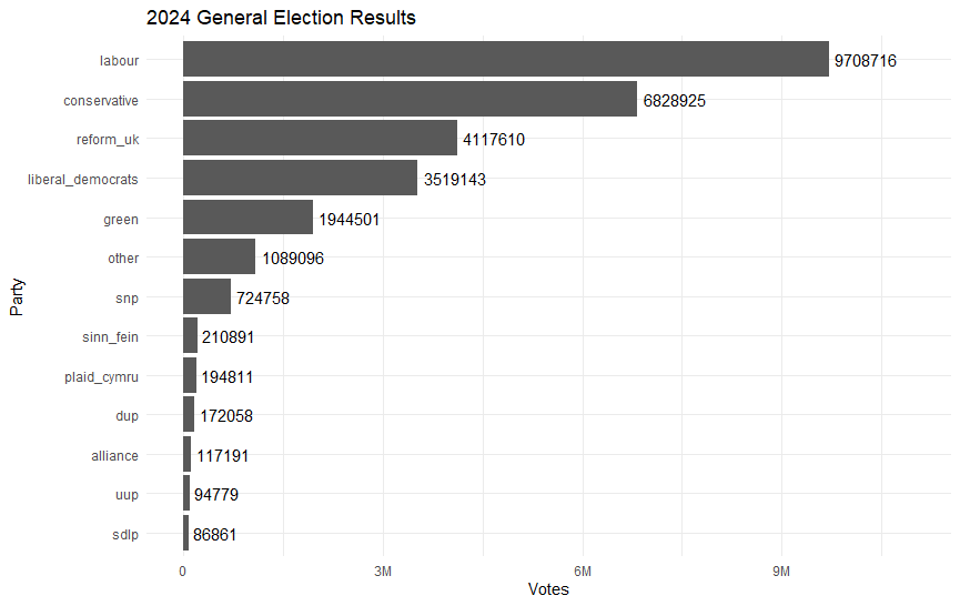
Which seems to match Parliament’s own vote count summary nicely, a snippet of which is shown here:
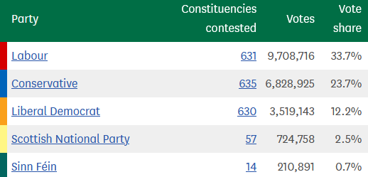
The same was true I checked the 2019 figures, as well as the number of unique constituencies contested in each year. All good.
Outstanding issues and usage guide
Nonetheless, there are plenty of issues we should be aware of when we get onto actually using this data for something. Aside from any mistakes I might have made, it turns out that consolidating many years worth of elections together is not as much of an exact science as one might hope.
The British electoral system, whilst remaining (almost exclusively) FPTP, has seen some changes over time in terms of which constituencies exist, their boundaries, the number of seats, which parties contest them, which parties even exist, the number of voters, who they were and so on. For the first few elections, up to 1928, the only women that were allowed to cast a vote at all were those who were over 30 years old and had some connection to property ownership. Before 1969 you had to be at least 21 years old to vote, irrespective of your sex.
The site I got the source data from call out a few idiosyncrasies that we should be aware of here when using this data – well worth a read – including that:
- Constituency boundaries changed following boundary reviews in 1945, 1948, 1955, 1974, 1983, 1997 and 2005 (Scotland)/2010 (rest of the UK).
- The definition of regions also changed over time.
- In older data, before 1950, there were at least 3 differences in how general elections worked that affect the data.
- Some seats returned two candidates instead of the standard 1 seat = 1 MP connection we have today. Data from these are thought to be less reliable. The Representation of the People Act 1948 brought this practice to a halt.
- Sometimes there was only one candidate, in which case the seat was uncontested. This meant no votes were cast at all, indicated by a -1 or -2 in the vote count data depending on how many MPs from the same party were returned.
- University seats existed, which were seats that graduates from a given university could vote for irrespective of where they lived. In the end I didn’t bring those into my data file, although they are available in the first tab of the 1918-2019 source Excel file. Again, the Representation of the People Act 1948 abolished these seats, and with that, no longer did certain university graduates get to have twice as many votes in general elections as the rest of us.
To that list I’d want to add at least that:
Firstly it would be incorrect to assume that the party that got the most votes for a given constituency in a given election won that seat seat. Logically, and in the vast majority of cases here in practice, yes that’s true – but unfortunately the source data categorises some of the minor parties into an “Other” category.
Whilst it’s rare, if it’s this “Other” column that contains the most votes for a constituency then there’s no way to tell in the data here whether that refers to a single “other” party, who then would have won the seat, or a combination of several parties in which case a “non-other” party may well have won.
One example of this can be seen in 2024 where in the BRADFORD WEST constituency we saw “Other” receiving 14,898 votes. This is the highest value for a supposed “party” in the data. But in reality it was Labour that won that seat by gaining 11,724 votes. Behind the scenes, and not available in this data, we can see that the “Other” result is a mix of three independent candidates – Muhammed Islam who actually only just lost with 11,017 votes and Akeel Hussain (3547) and Umar Ghafoor (334).
In fact the 2024 source data does reveal who won each seat, but the source data from all the previous years did not include that field so I felt compelled to drop it for now.
Secondly, the total votes column I created is non-additive. It tells you the total number of votes cast in that constituency for that election for all parties combined. The same figure is repeated on each party’s row for that constituency and election. This makes it easy to work out metrics such as % vote share within the seat, but if you were to try and sum total_votes across the whole dataset you would dramatically overstate the number of votes cast. However it would be safe to sum the party-specific votes field to get the overall total vote count.
