Geographic location analysis has been an important subset of data analysis since time immemorial. One of the most famous examples from times past is the visualisation that John Snow created in response to an outbreak of cholera almost 170 years ago.

That dataviz led to an action – the disabling of a water pump that was a source of the outbreak – that probably saved lives.
Perhaps the stakes are a little lower for most analysts’ day-to-day work, but spatial analysis can nonetheless reveal a ton of insights otherwise hard to discern. And now the majority of the world’s population appears to be happy to carry around what is often basically an internet-connected GPS tracker – i.e. your smartphone – the amount of this style of data that exists has never been more abundant, which is also true for most other forms of data to be fair.
But location data is not always the easiest type of data to work with. If we imagine the type of location data that is sometimes quietly sucked up as you innocently play your phone game at home for instance, the end recipient might end up with hundreds of slightly different coordinates that represent your exact longitude and latitude as you wander through the rooms of your house.
The fine distinction between these precise coordinates may be important for some use-cases. But for anything I’ve really needed needed to do with this type of data, I just wanted to determine which places in general appear to be important to the person concerned. I haven’t yet had cause to care how long a person spends scrolling their phone specifically in their bathroom, fun as that would be to know.
Dealing with tons of unnecessarily detailed coordinates can also introduce a lot of time-consuming computational complexity. Perhaps I want to calculate the travel time between the various places a person visits in their day. The vast majority of their coordinates might be narrowly confined to their home and place of work perhaps. It would be wasteful for me to calculate the distances between every pair of points if all I really cared about was how far they they lived from their workplace work.
And then there’s a privacy aspect. If you do not need to keep location data at an extremely detailed granularity then you shouldn’t. Even if you and everyone you know is perfectly ethical and trustworthy, there there’s always the risk of it leaking out one way or another. Summarising the data a bit might also save you storage cost and space.
In these scenarios then we often want to aggregate the set of longitude/latitude coordinates so as to be able to say “this set of 1000 closely knit coordinates can roughly be represented by a single location A vs this set which can be represented by location B”.
Aggregating latitude and longitude coordinates via the H3 system
H3 is a “discrete global grid system” that can be used to do exactly that kind of aggregation at a variety of different grains.
The basic way it works is by dividing the world up into a hexagonal grid. Each hex within the grid has a unique cell ID. And so you can assign individual longitude and latitude coordinates to their respective hexagonal cells. Then you can use their cell IDs to aggregate and work with an often-more-suitable reduced level of granularity.
Here’s what it promises:
Indexed data can be quickly joined across disparate datasets and aggregated at different levels of precision. H3 enables a range of algorithms and optimizations based on the grid, including nearest neighbors, shortest path, gradient smoothing, and more.
Why hexagons? That’s explained in their documentation.
A basic grid system designed to encompass locations can most simply be represented by a polygon that tessellates regularly. Triangles, squares and hexagons all do this. But hexagons have the advantage that all neighbouring hexes to a home hex are the same distance apart. This isn’t the case for triangles or squares. This makes analysing movement between hexes easier.

The ring of neighbours to a hexagon also approximates a circle which can be useful, plus they’re better at filling arbitrary spaces than the other candidates mentioned.
How large are the hexagons? Well, that’s up to you. They’re available in 16 resolutions, with higher-numbered resolutions meaning that the hexagons are smaller, and hence more plentiful and a more precise representation of a given coordinate. Each higher resolution has cells that are 1/7th of the area of a cell in its parent’s resolution.
For efficiency you might then pick the lowest resolution that still provides enough detail to do what you need.
Here’s an example from Uber’s blog post on the subject – it was their team that came up with the H3 system – showing how a given area can be subdivided up into ever-smaller hexagons depending on the resolution you choose.
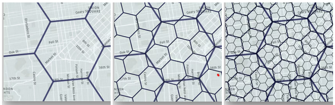
You can’t quite fit 7 small hexagons into 1 big one perfectly, but to the extent that it’s close to being the case you can treat H3 as being a hierarchical boundary system. Functions exist within its typical implementation to move up and down the resolution chain.
You can interactively play around with the reality of what these resolutions reflect using this Streamlit app.
The H3 documentation also gives the average area that the hexes at each resolution encompass.
| Resolution | Average Hexagon Area (km2) |
|---|---|
| 0 | 4,357,449.416078381 |
| 1 | 609,788.441794133 |
| 2 | 86,801.780398997 |
| 3 | 12,393.434655088 |
| 4 | 1,770.347654491 |
| 5 | 252.903858182 |
| 6 | 36.129062164 |
| 7 | 5.161293360 |
| 8 | 0.737327598 |
| 9 | 0.105332513 |
| 10 | 0.015047502 |
| 11 | 0.002149643 |
| 12 | 0.000307092 |
| 13 | 0.000043870 |
| 14 | 0.000006267 |
| 15 | 0.000000895 |
Anyway, let’s take a quick look at how we might use this system.
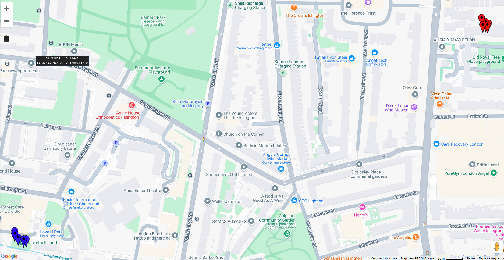
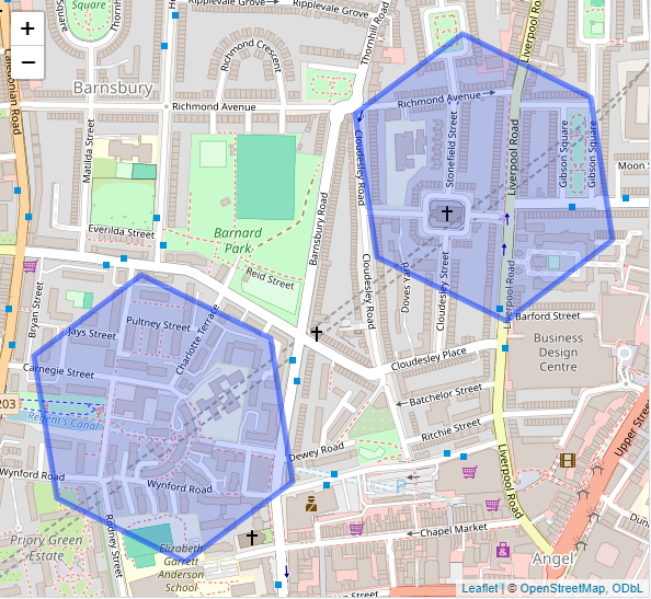
Imagine a scenario where you have tracked someone to a set of coordinates represented by the red markers at the top right and blue markers at the bottom left of this map.
An interactive version of this map can be seen here.
Perhaps the red markers represent where they live and the blue is their phone’s location whilst playing a game of basketball in the local court.
But the precision of these coordinates is too much. The individual differences between the red markers aren’t interesting to me so I want to aggregate them up into a suitably sized hex.
Working with H3 in Snowflake
Let’s start off by using the Snowflake database, which conveniently has a set of H3 functions built into it. They can work either using Snowflake’s existing GEOGRAPHY data type, or, as I will show below, with raw latitude and longitude coordinates.
First up, let’s get the coordinates of at least some of those red and blue markers into Snowflake. Here we use a CTE to create a data structure with simple latitude and longitude columns:
with coordinates as(

    select $1 as latitude,
      $2 as longitude

    from values
      (51.537149481653, -0.10615450282663),
      (51.53707273735, -0.10613572736352),
      (51.537107630668, -0.10608607221501),
      (51.53707273735, -0.10605526109308),
      (51.537089870011, -0.10603720765571),
      (51.534816530538, -0.11437627544823),
      (51.534743119185, -0.1143172668499),
      (51.53472643477, -0.11422070732536))

select *
from coordinates;
In later SQL, whenever I refer to coordinates that’s the CTE I’m talking about.
OK then, how do I convert each coordinate into the ID of the H3 hexagon it’s in?
It’s very easy as it happens. Snowflake has a built-in function for that called H3_LATLNG_TO_CELL_STRING. There are other similarly named variants of this command if you’re working with GEOGRAPHY objects or want an integer as opposed to the more common hexadecimal identifier of the hex.
When requesting the H3 hexagon you will want to specify the resolution. As noted above, higher resolution numbers reflect smaller hexes.
For my example here, let’s say I’m fine with hexagons that average an area of about 0.1 square kilometres each. That’s resolution number 9.
So:
select
latitude,
longitude,
H3_LATLNG_TO_CELL_STRING(latitude, longitude, 9) as h3_hex

from coordinates;
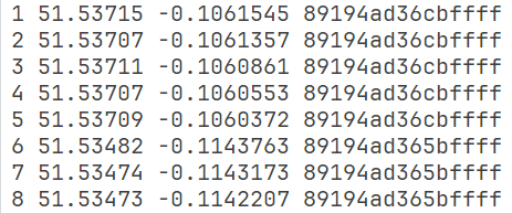
gives me an output like:
| LATITUDE | LONGITUDE | H3_HEX |
|---|---|---|
| 51.537149481653 | -0.10615450282663 | 89194ad36cbffff |
| 51.537072737350 | -0.10613572736352 | 89194ad36cbffff |
| 51.537107630668 | -0.10608607221501 | 89194ad36cbffff |
| 51.537072737350 | -0.10605526109308 | 89194ad36cbffff |
| 51.537089870011 | -0.10603720765571 | 89194ad36cbffff |
| 51.534816530538 | -0.11437627544823 | 89194ad365bffff |
| 51.534743119185 | -0.11431726684990 | 89194ad365bffff |
| 51.534726434770 | -0.11422070732536 | 89194ad365bffff |
You can see that the 8 distinct sets of lat/long coordinates have been aggregated to just 2 hexes, “89194ad36cbffff” and “89194ad365bffff”.
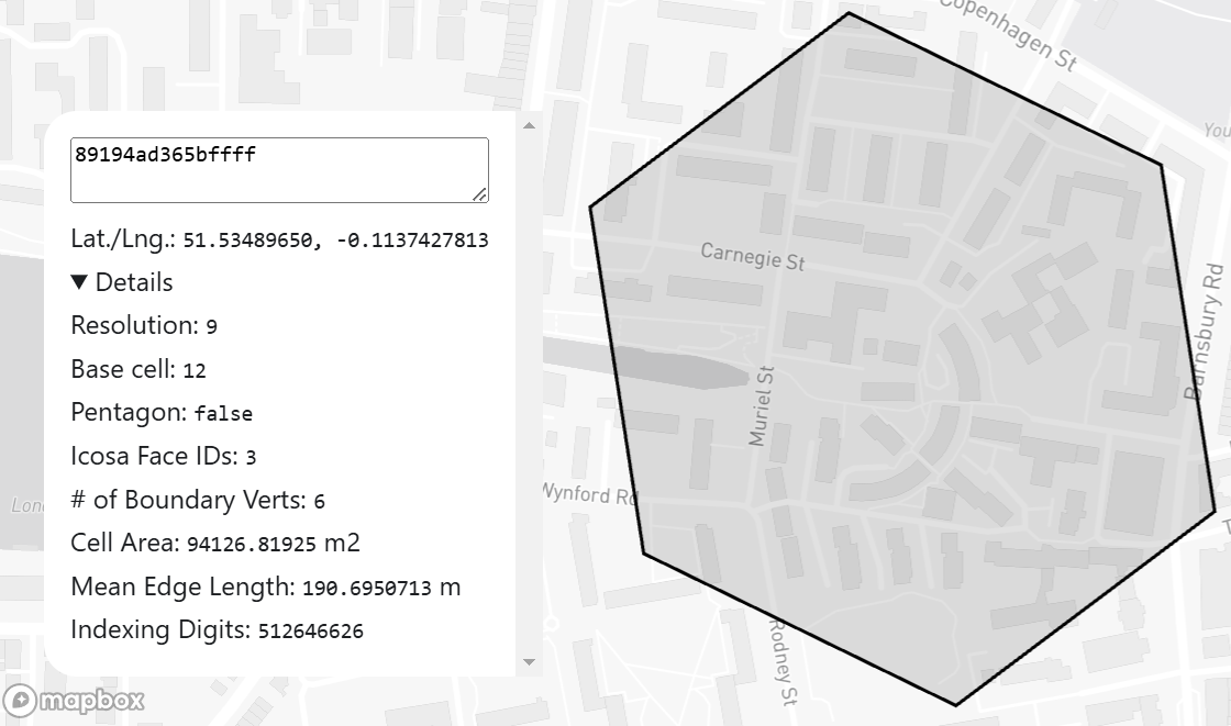
To quickly visualise the scope of the hexes concerned you can use the gadget on the top of the H3 homepage that lets you type in a H3 hex code and see where on a map it corresponds to.
For 89194ad365bffff, we can see that it does indeed include the Muriel Street / Carnegie Street area that’s found around the basketball court in my original map.
That was simple enough! But what if I’d made the wrong decision about the resolution? Perhaps I don’t want quite this level of precision. Well, the function H3_CELL_TO_PARENT converts a H3 cell at one resolution to the less-granular cell that it would be held within at a lower resolution.
Let’s convert my resolution 9 hex IDs to those of a lower resolution, resolution 6.
select latitude,
longitude,
H3_LATLNG_TO_CELL_STRING(latitude, longitude, 9) as h3_hex_r9,
H3_CELL_TO_PARENT(h3_hex_r9, 6) as h3_hex_r6
from coordinates;
Now all my coordinates are in one, much larger, hex, shown here as column h3_hex_r6.
| latitude | longitude | h3_hex_r9 | h3_hex_r6 |
|---|---|---|---|
| 51.537149481653 | -0.10615450282663 | 89194ad36cbffff | 86194ad37ffffff |
| 51.537072737350 | -0.10613572736352 | 89194ad36cbffff | 86194ad37ffffff |
| 51.537107630668 | -0.10608607221501 | 89194ad36cbffff | 86194ad37ffffff |
| 51.537072737350 | -0.10605526109308 | 89194ad36cbffff | 86194ad37ffffff |
| 51.537089870011 | -0.10603720765571 | 89194ad36cbffff | 86194ad37ffffff |
| 51.534816530538 | -0.11437627544823 | 89194ad365bffff | 86194ad37ffffff |
| 51.534743119185 | -0.11431726684990 | 89194ad365bffff | 86194ad37ffffff |
| 51.534726434770 | -0.11422070732536 | 89194ad365bffff | 86194ad37ffffff |

Of course if you’re working from raw coordinates you can simply convert to resolution 6 directly. This might give you slightly different, perhaps superior, results because of the issue that you can’t quite fit 7 children hexes into 1 big parent hex, even if you nearly can.
Nonetheless, in this case one would get exactly the same results either way, verifiable with this code:
select latitude,
longitude,
H3_LATLNG_TO_CELL_STRING(latitude, longitude, 9) as h3_hex_r9,
H3_CELL_TO_PARENT(h3_hex_r9, 6) as h3_hex_r6,
H3_LATLNG_TO_CELL_STRING(latitude, longitude, 6) as h3_hex_r6_direct,
from coordinates;
Another couple of H3 functions that caught my eye include:
H3_GRID_DISTANCE, which gives you the distance between two H3 cells based on their IDs. So we could run:
SELECT H3_GRID_DISTANCE('89194ad36cbffff' , '89194ad365bffff')
which gives the result ‘2’.
This tells us that getting between the two resolution 9 cells identified above would involve two hops. That’s to say that the hexagons are not immediate neighbours, but that they are only 1 hex away from each other at this resolution.
And which hex would that one obstructing hex be? Here’s how to get the path between two hexagons using H3_GRID_PATH:
select H3_GRID_PATH('89194ad36cbffff' , '89194ad365bffff')
This returns the array:
[
  "89194ad36cbffff",
  "89194ad3653ffff",
  "89194ad365bffff"
]
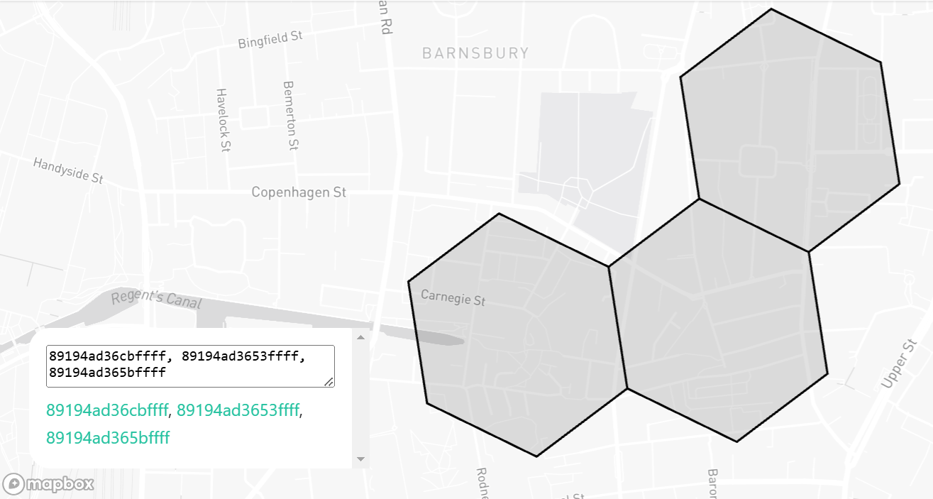
This shows us that one efficient way to get from hex cell ID 89194ad36cbffff to 89194ad365bffff involves going through hex cell ID 89194ad3653ffff – confirming that the two original hexes are indeed 2 hops away from each other.
Visualised via the h3geo tool this looks like:
Working with H3 in R
Let’s switch now to another language, R.
There’s a few R libraries out there that work with H3 data. I’m going to use the one simply named h3, details of which are available here. It’s a one-step solution, no need to install any separate H3 C library or other extraneous items which some of the other solutions require.
Right now though this library isn’t available on CRAN. Instead you can install it using the remotes package, like this:
install.packages("remotes") # only if you haven't already installed remotes
remotes::install_github("crazycapivara/h3-r")
Now start off by loading the library and, once again, creating a simple dataframe to hold our example latitude and longitude coordinates.
library(h3)

coordinates <- data.frame(
  latitude = c(
    51.537149481653,
    51.53707273735,
    51.537107630668,
    51.53707273735,
    51.537089870011,
    51.534816530538,
    51.534743119185,
    51.53472643477
  ),
  longitude = c(
    -0.10615450282663,
    -0.10613572736352,
    -0.10608607221501,
    -0.10605526109308,
    -0.10603720765571,
    -0.11437627544823,
    -0.1143172668499,
    -0.11422070732536
  )
)
This library’s equivalent to Snowflake’s H3_LATLNG_TO_CELL_STRING function is geo_to_h3. We can convert our above coordinates to the same resolution 9 hex IDs like this:
library(dplyr)

coordinates <- coordinates |>
  mutate(h3_hex_r9  = geo_to_h3(coordinates, res = 9))

# Print the dataframe
print(coordinates)
The output is as expected:
There’s a good deal of other functionality in this package worth exploring (and, to be fair, the within the Snowflake function library too).
For instance, if you have the R package sf installed you can convert a H3 hex ID into a polygon corresponding to its boundaries.
Here then would be the two hexes represented in my resolution 9 coordinates data as a sf polygon.
hex_boundaries <- coordinates |>
  select(h3_hex_r9) |>
  distinct() |>
  mutate(r9_polygon_sf_object =  h3_to_geo_boundary_sf(h3_hex_r9))

Now you have the boundaries, you can easily visualise them on a map within your analysis via any library that can work with sf objects.
Here for example is a very simple example using the leaflet library.
library(leaflet)

map <- leaflet() |>
  addTiles() |>
  addPolygons(data = hex_boundaries$r9_polygon_sf_object)
Let’s superimpose our initial lon/lat coordinates on the map to check that they do in fact come from the hexagons represented
map |>
  addMarkers(data = coordinates, lng = ~longitude, lat = ~latitude)
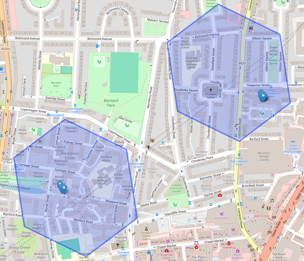
Perfect!
Now we visualised it, we can see that the two polygons corresponding to this person’s location data are a gap of about polygon away. But we don’t have to do this by eye of course. The h3_distance function expresses the grid distance between two H3 hexes, similarly to the Snowflake H3_GRID_DISTANCE function.
In this case we could have run:
h3_distance("89194ad36cbffff", "89194ad365bffff")
to get the result of 2, indicating the two hexes are two hex-jumps away from each other.
Or perhaps you need something like the opposite type of analysis – which cells are near to my current hex? The below gives me the IDs of all the hexes that are adjacent to the one with ID 89194ad36cbffff:
k_ring("89194ad36cbffff", radius = 1)
…which provides this list of of the 6 adjacent cell IDs at the same resolution (as well as the original hex’s cell ID itself):
"89194ad36cbffff" "89195da6b37ffff" "89195da6b27ffff" "89194ad3653ffff" "89194ad36cfffff" "89194ad36c3ffff" "89194ad36dbffff"
These, as with any other collection of H3 cell IDs, could be visualised in the same sort of way as we saw above:
k_ring("89194ad36cbffff", 1) |>
  h3_to_geo_boundary_sf() |>
  leaflet() |>
  addTiles() |>
  addPolygons()

