Using R to run many hypothesis tests (or other functions) on subsets of your data in one go

It’s easy to run a basic hypothesis test in R, once you know how. For example, if you’ve a nice set of data that you know meets the relevant assumptions, then you can run a t test in the following sort of way . Here we’ll assume that you’re interested in comparing the differences in the number of apples eaten between people, based on which group they’re in, from an imaginary “foods eaten” experiment dataset.

t.test(apples_eaten ~ group, data = foods_eaten)

The above uses the default values for hypothesis type, expected difference, confidence level et al. but these are all configurable by various parameters should you need to do so.

The default output looks something like this:

Welch Two Sample t-test

data: apples by group
t = 0.033192, df = 76.123, p-value = 0.9736
alternative hypothesis: true difference in means is not equal to 0
95 percent confidence interval:
-2.950128 3.050128
sample estimates:
mean in group a mean in group b 
9.05 9.00

Here we can see that the difference in means does not seem significant by pretty much any definition; the most obvious indicator being that the p-value is way above the traditional – if increasingly controversial –  “significance” cutoff of 0.05.

This output nice enough for interactive use if you’re analyzing a single variable from an experiment or two. But, let’s say your dataset actually includes the results of several experiments, several outcome variables, or some other scenario where you want to conduct multiple hypothesis tests in one go. Do you really want to run the above command many times and manually collate the results into a nice table to let you see a quick overview of results? Well, of course not! R, being your servant rather than your master, should run them all for you and output the results into a nice clean table, right?

First up though, you should probably consider why you’re doing this. Running multiple unadjusted t-tests for different groups within the same data is often a very bad idea. Per usual, xkcd provides an awesome explanation as to why.

If you’re looking at the differences between multiple subgroups in one experiment, you should often prefer, for example, an ANOVA test to several t-tests. This helps to avoid inflating the chances of a type 1 error, and falsely concluding you found an effect when in reality there isn’t one. I have also seen some instances of people running (unadjusted) multiple t-tests after an ANOVA has reported an effect in order to try and determine between which of the groups in the ANOVA the difference is significant in –  but this holds the same sort of danger. In that case, there’s plenty of standard post-hoc tests it would be more legitimate to use instead – Tukey’s HSD test for instance is similar to a t test, but contains adjustments to reduce the error rate.

Anyway, enough with the theoretical warnings. Perhaps you do have a valid use case. Or perhaps you realise that the below technique really allows you to run many different kind of functions that aren’t t tests on a dataset. These may be other types of hypothesis tests, or functions entirely unrelated to such testing. If this is the case, you can think of this as a template.

Let’s think through the mechanics of what we want to do. Let’s take a contrived (and fake) scenario in which we conducted 2 experiments, each involving 2 sets of people, a control and a test group. We measured how many of various different types of fruits and vegetable they ate. We’re interested in whether each group within an individual experiment differed in terms of the mean average of each type of fruit eaten.

Here’s a few rows of the sample data this non-existent experiment generated.

experiment_number	group	person_number	apples	bananas	carrots	dandelions	eggplant
Experiment 1	a	1	1	3	3	3	1
Experiment 1	a	3	1	1	3	3	5
…
Experiment 1	b	103	2	5	3	5	2
Experiment 1	b	104	8	1	3	1	2
…
Experiment 2	c	7	19	5	8	0	3
Experiment 2	c	12	4	5	6	1	0
…
Experiment 2	d	111	16	3	6	0	5
Experiment 2	d	113	12	3	4	4	0

Our goal here, for the sake of argument, is to perform a t test for each experiment (identified by the “experiment number” column), comparing the 2 relevant groups of participants (the “group” column) in terms of how many apples they ate. Then, separately, on how many bananas they ate, and so on through the other edibles. Then we want to move on to experiment 2 and repeat the same exercise, until we have a hypothesis test result for each experiment on each of the foodstuffs. Yes, I know, if this was a real analysis, we’d need to revisit the above xkcd cartoon and think hard about whether this is the appropriate design for analysing the experiment.

But, that aside, this means we need to:

1. Select only the group of data that has the first experiment_number, i.e. anything with experiment_number = Experiment 1 here.
2. Select the first outcome variable of interest (apples)
3. Run a t test on it, comparing participant groups against each other (here group a vs group b).
4. Record the results of that t test (let’s say the t statistic, the p value, and the estimated difference in means) as a row in a results table
5. Go back to step 2, but moving to the next outcome variable, here examining bananas instead of apples, until we’ve tested all the outcome variables.
6. Go back to step 1, moving to the next experiment number, i.e. Experiment 2, and repeating the whole process again.

In this dataset, 2 experiments with 5 outcomes, that’s 10 t-tests. I don’t want to look at 10 of the default outputs for R’s t.test function, thank you. I’d prefer a result that looks something like this…

experiment_number	food_type	estimated mean of first group	estimated mean of second  group	t statistic	p value
Experiment 1	apples	9.05	9	0.03	0.97
Experiment 1	bananas	2.5	2.875	-1.02	0.31
…
Experiment 2	dandelions	2.16	2.84	-1.76	0.08
Experiment 2	eggplant	3.2	3.66	-0.86	0.39

…where we’ve a table, or “dataframe” as R calls it, showing 1 row per t test with the most relevant statistics.

OK, let’s go, building it up step by step. Being R, of course there’s a multitudinous variety of ways we could do this. Being a tidyverse fan, I’m going with what could be described as a dplyr approach. We’re going to need to install and load the following libraries to use this method.

• tidyr: to get the data into a “tidy” format.
• dplyr: to manipulate the data into the groups you wish to hypothesis test on.
• broom: to tidy up the results of the default R t.test output into a nice tabular format

So, load up these libraries, remembering to install the packages first if you’ve not already done so, as below.

install.packages("tidyr") # only needed if you didn't ever install tidyr
install.packages("dplyr") # only needed if you didn't ever install dplyr
install.packages("broom") # only needed if you didn't ever install broom

library(tidyr) # to get data into "tidy" format
library(dplyr) # to manipulate data
library(broom) # to tidy up the output of the default t test function.

Step 2 is to transform the data table of experiment results from a “wide” format to a “long” format.

Many tidyverse functions, and much of R in general, works better with long data. We know our lowest level of grouping – i.e. the granularity we want to conduct our tests at – is at a per experiment per outcome variable level. For example, we’ll need to group all of the “apples” data for “experiment 1” together so we can analyse it with an individual test.

If we’re going to group then the experiment number and the outcome variable type should probably be individual columns. The experiment_number already is. But the outcome variables aren’t – they each have their own column. We thus want to get from this situation: 1 row per person who participated in the experiment…

experiment_number	person_number	group	apples	bananas	carrots
1	1	a	1	2	3
2	7	c	19	24	6

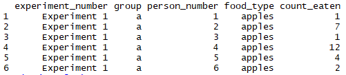
…to this format – 1 row per outcome variable per person. Note how the experiment number, group, and person number are repeated down the rows, in order to keep track of whose apples outcome the row concerns.

experiment_number	group	person_number	food_type	count_eaten
Experiment 1	a	1	apples	1
Experiment 1	a	1	bananas	2
Experiment 1	a	1	carrots	3
…
Experiment 2	c	7	apples	19
Experiment 2	c	7	bananas	24
Experiment 2	c	7	bananas	6

We’re using a “food_type” column to record which outcome variable we’re talking about (apples vs bananas), and the “person_number” column to ensure we keep track of which entries belong to the same person:

This “unpivoting” is a perfect use-case for dplyr’s gather() function. Here we go:

results <- gather(data, key = "food_type", value = "count_eaten", -experiment_number, -person_number, -group)

The "key" parameter of the command lets us set the name of the column that will store the name of the outcome variable we're looking at. The "value" parameter lets us set the name of the column that will store the actual result obtained by the participant for the specified outcome variable.

Where we see "-experiment_number, -person_number, -group" at the end of the function call, that's to tell it that – because experiment number, person number and group are not outcome variables – we don’t want to collapse their contents into the same column as the count of apples, bananas etc. We need these variables to be replicated down the list to know which experiment, person and group the respective outcome variable was obtained from.

Note the minuses in front of those variable names. This means “don’t unpivot these columns’. If you only had  a few columns to unpivot, you could instead write the names of the columns you do want to unpivot there, without the minuses.

Let’s check what “results” now looks like, by typing head(results).

OK, that looks very much like what we were aiming for. Onto the next step!

Now we need to ensure our analysis is only carried out using the data from a single experiment for a single outcome. Our outcomes here are the food type counts. For example, we want to consider the data from Experiment 1’s apples outcome separately from both Experiment 1’s bananas outcome, and Experiment 2’s apples outcome. In other words, we want to group the data by which experiment it’s from and which food type it’s measuring.

Handily, dplyr has a group_by function. Pass in the data you’re working with, and the names of the columns you want to group it by.

results <- group_by(results, experiment_number, food_type)

Checking the  head of the results now looks pretty similar to the previous step, only this time the output tells you, quite faintly, near the top, that we've grouped by the appropriate variables.

Now, it’s time to do the actual t tests!

First of all, remember that we don’t want a bunch of those verbose default t.test outputs to work with. We want a nice table summarising the most important parts of the test results. We thus need to make the key parts of t test output “tidy“, so it can be put into a table, aka dataframe.

How to tidy the results of a hypothesis test? Use broom. Horray for R package names that attempt some kind of pun.

Let’s first take a moment to see how tidying works with a single t test, run in the conventional way.

Here’s the output of the default t.test function looking at the apples outcome of experiment 1. First I constructed a dataframe “exp1_apples_data”, which contains only data about apples, from experiment 1. Then I ran the standard t.test – being explicit about many of the options available, although if you like the defaults you don’t really need to be.

exp1_apples_data %>%
  select(group, person_number, apples)

t_test_results <- t.test(apples ~ group,
       data = exp1_apples_data,
        alternative = "two.sided",
        mu = 0,
        paired = FALSE,
        var.equal = FALSE,
        conf.level = 0.95)

t_test_results

This outputs:

Now, if we apply the tidy() function from the broom package to the results of the t test, what do we get?

tidy(t_test_results)

Outputs:

Yes, a nice tidy 1-row summary for the results of the t test. Comparing it to the default output above, you can see how:

• field “estimate1” corresponds to the mean in group a
• “estimate2” corresponds to the mean in group b (and the “estimate” field corresponds to the difference between the mean in group a and b)
• “statistic” corresponds to the t statistic
• “p.value” corresponds to the p-value
• “parameter” corresponds to the degrees of freedom
• “conf.low” and “conf.high” correspond to the confidence interval
• “method” and “alternative” record the type & nature of the test options selected

So now we have a set of grouped data, and a way of producing t test results in in a tabular format. Let’s combine!

For this, we can use the dplyr function “do“. This applies what the documentation refers to as an “arbitrary computation” (i.e. most any function) to a set of data, treating each of the groups we already set up separately.

The first parameter is the name of the (grouped) dataset to use. The second is the function you want to perform on it.

results <- do(results, tidy(t.test(.$count_eaten ~ .$group,
                 alternative = "two.sided",
                 mu = 0,
                 paired = FALSE,
                 var.equal = FALSE,
                 conf.level = 0.95
                 )))

 

Note that you have to express the t test formula as .$count_eaten ~ .$group rather than the more usual count_eaten ~ group. Inside, the do() function, the . represents the current group of data, and the $ is the standard R way of accessing the relevant column of a dataframe.

What do we have now? Here's the head of the table.

Success! Here we see a row for each of the tests we did –  1 per experiment per food type –  along with the key outputs from the t tests themselves.

This is now just a regular data frame, so you can sort, filter, manipulate or chart as you would with any other dataset. Figuring out which of your results have  p value of 0.05 or lower for instance could be done via:

filter(results, p.value <= 0.05)

Below is a version where the commands are all pieced together, using the pipe operator.  That’s likely easier to copy and paste should you or I have a need to do so. Do remember that this is applicable, and perhaps more often actually theoretically valid, to the world outside of t tests.

The tidy() command itself is capable of tidying up many types of hypothesis tests and models so that their results appear in a useful table format. Beyond that, many many other functions that will return something coercible into a row of a dataframe or as an item in a R list, so will work.

results %>%
  group_by(experiment_number, food_type) %>%
  do(tidy(t.test(.$count_eaten ~ .$group,
                 alternative = "two.sided",
                 mu = 0,
                 paired = FALSE,
                 var.equal = FALSE,
                 conf.level = 0.95
                 )))