Sometimes we don’t have the luxury of running a gold-standard randomised controlled trial when wanting to understand the effect of some intervention on some population. Perhaps the required experiment would be unethical, too costly, or otherwise unfeasible. Or maybe the powers that be just never thought about doing a proper experiment, but yet want to understand something about the impact.
A dangerously naïve approach would be to just forget that you didn’t assign “participants” to treatments randomly and compare those who happened to get the intervention vs those who didn’t. In terms of creating descriptive statistics that works, but it can’t tell you anything at all about the effectiveness of the intervention. One key reason being that there’s usually some reason why some people got a given intervention – and maybe that reason also happens to relate to the outcome you’re measuring.
As a simple example of the challenge here, imagine older folk are more likely to go ask their doctor for a certain medication than younger folk are. If more of the people that took the medication end up dying, how could we know whether the medication is deadly, or it’s just the “being older” that’s causing extra mortality?
The field of causal inference exists in part to help statisticians address these thorny issues rather than just throw their hands up in the air and give up. One common technique used is called “matching“. For once, this is roughly what it sounds like it would be in common English.
What is matching?
A simplistic version of the approach to the above medication example might work as follows:
- For each person who took the medication, find another person that is similar to them in terms of all of the attributes that relate to the outcome except that they didn’t take the medication. In the above simple case, that would mean that they’re similar in age. These are the matches.
- If there’s any participants that can’t be matched up to someone similar in the other group then ask them to leave.
- At the end of this, you end up with two groups, one of which took the medication and one of which didn’t – but now their distribution of ages is similar.
- If there are still mortality differences between these groups then you can be sure that they’re not due to the fact that the people in one group tend to be older than the people in the other.
In reality you are likely going to match on more than one variable. For instance if you think that both age and sex might matter to the outcome of your treatment, you’ll be looking to match a female aged 65 who had the medication with a female aged around 65 who didn’t take it.
It should be noted that there are many different approaches to matching out there. Some variations include:
- Instead of throwing participants out of the analysis and losing their information entirely you might choose to re-weight their contribution to the results. If there’s a lack of younger folk in the treatment group, maybe you upweight their contribution to the outcome to compensate for that difference.
- You might also have differing rules about how close a match needs to be to be legitimate, as well as what to do about participants with no obvious matches.
- There are also different algorithms to consider when deciding what the “distance” between participants is; for example is a female aged 65 “closer” to a male aged 64 or a female aged 20?
- You can either match “without replacement” meaning once someone has been matched with another person they can’t be matched with a third person no matter how similar they are. Or you might choose a “with replacement” approach where if the same person is a close match to multiple other people they might be used several times.
Some of these decisions may be domain dependent, but hopefully the general idea of “what is matching?” is clear enough.
It should be noted that matching is not a free lunch. If you can realistically run a RCT then you should usually do so! Articles on the limitations abound, but a couple of simple ones include:
- You must “magically” know what all the important variables that affect the outcome you care about are, and be able to measure them accurate. Sure, in the above example you have people’s ages, but what if it’s actually their income that matters to the outcome? The resulting matched groups will not necessarily be similar in terms of income, risking false conclusions.
- Sometimes people that choose a treatment may be very different than those who do. If only 60 year olds tend to take the treatment and the only comparison you have comes from 20 year olds then there’s nothing you could possibly match up there. In general there’s a compromise to be made between finding close matches, and including data from as many people as possible. You can’t say much about the effect of your treatment on folk that were excluded from your analysis, potentially limiting generalisability.
Most matching algorithms struggle with large or multi-group samples
Whilst matching is conceptually fairly simple as far as these things go – in that the non-analysts I speak to tend to grasp the idea reasonably well – it’s actually computationally very challenging. Once we have decided how we’re going to decide how similar one participant is to another, which potentially involves a lot of different variables, we then need to make the matches. In the worst – but most optimal in terms of match quality – case this might mean comparing every single participant with every single other participant that they could be matched with, and somehow figuring out the best combinations. Participant A might be similar to participant B. But so is participant C, so you ideally want to figure out whether if you match C with A and D with B that’s better than A-B and C-D.
Basic modern-day computers can do that swiftly enough if maybe you’ve got a few hundred or thousand participants to consider. But if you get into much bigger numbers it becomes a struggle. I’ve sometimes left my computer running overnight to get it to process matches within a few hundred thousand people, or felt compelled to take smaller random samples of the original data so that I can match it in a reasonable time frame.
Another limitation of most of the approaches I’ve seen is that they assume that there are two groups of interest. This is often true – in my above example, people either took the medicine or they didn’t. That’s akin to a treatment group and a control group. But what about if there are actually several treatments for a given ailment – some people took treatment A, others took treatment B and some took neither? If your goal is to compare A vs B vs doing nothing then you need to create matches between people from all 3 groups.
A rough and ready way to do this – one I must confess I’ve used in the past – is to for example match “no treatment” to “took A”, and separately “no treatment” to “took B”, and then combine the both sets of results. But there’s nothing in that approach that matches people in “took A” to those in “took B” so they may in fact not be all that similar to each other. That said, my experience is that the results are often reasonably OK with big samples.
The quickmatch solution
One solution to the computational time and power needed to process large samples, as well as the common inability to have compare than two groups issues with matching have been addressed in a paper by Fredrik Sävje, Michael J. Higgins and Jasjeet S. Sekhon called “Generalized full matching and extrapolation of the results from a large-scale voter mobilization experiment“.
The paper describes a matching method that can work speedily with very large samples and any number of treatment groups. The matching results are obviously not going to be theoretically “optimal” when compared to certain slower and more limited methods for a dataset that could realistically be processed by either. But they are close, and there is a reassuring hard limit on how “suboptimal” it can be. My personal experience is that they are actually very close to optimal in practice, actually better than some of my other, occasionally slightly hacky, attempts. But what this approach adds is actually making it feasible to use matching in big and complicated samples in the first place. Matching exercises that take hours with other methods takes seconds or minutes here.
The example the paper uses to demonstrate how it works is a voter-mobilisation experiment that includes 6 different arms and nearly 7 million potential participants. It would be practically impossible to use matching at this scale on my computer using many of the other methods I’ve dabbled with.
What I really love about this paper is that the authors made the data and code behind the experiment analysis available for download. And I don’t mean they wrote “data is available upon request” (which apparently most of the time turns out to be untrue). You can literally download it at will here. Reading the paper alongside the code was great in helping me learn how I can apply their work to my own. I also want to extend extra gratitude to Fredrik Sävje who when I bothered him with questions via Github was very quick to respond with generous and helpful answers. It was a great experience.
On which note, the authors have created an R library called quickmatch that allows us to easily incorporate their approach within our own projects, which you can download via CRAN, or see the code on Github.
Below I intend to share some information about how one can use it, surmised from their paper, documentation and the conversations with Dr Sävje I mentioned above. All mistakes are of course my own. If you’re interested in leveraging their approach, I certainly would recommend reading their paper first.
Using quickmatch
Creating an illustrative dataset
First let’s create a deliberately unbalanced dataset to use as an example. The hypothetical example this represents is as follows:
- There are 100,000 potential participants in group A and the same number in group B. You could imagine this as one group that had some intervention and one that didn’t – but collated from non-randomised observational data.
- Although my example contains only these two “treatment groups”, note that one of the advantages of the
quickmatchpackage we’re using here is that it can handle any number of these groups – a group C and D would be no problem to work with in exactly the same way as below. - People in group A tend to be younger, shorter and more likely to be male that people in group B.
- The outcome we’re interested in is a score of some imaginary test. We’re deliberately setting this up such that the score is associated with the age and height of the participant (and nothing else). But, importantly, the scores are not structurally different between the participants in group A and B – although there’s some random noise added in the name of e.g. sampling or measurement error, so they won’t be identical.
The resulting table format we’re want for using with quickmatch is the typical R hypothesis test format: one row per participant, with a field indicating which group they’re in. Here’s some code that generates this kind of data with the above requirements.
library(tidyverse)

data <- as_tibble(c(rep("a", 100000), rep("b", 100000))) |>
  rename(group = value)

data <- data |>
  mutate(
    id = row_number(),
    age = if_else(group == "a", rnorm(nrow(data), mean = 50, sd = 10), rnorm(nrow(data), mean = 60, sd = 10)),
    height_cm = if_else(group == "a", rnorm(nrow(data), mean = 150, sd = 20), rnorm(nrow(data), mean = 160, sd = 20)),
    sex = if_else(group == "a", if_else(rbinom(nrow(data), size = 1, prob = 0.4) == 1, "F", "M"), if_else(rbinom(nrow(data), size = 1, prob = 0.6) == 1, "F", "M")),
    score = rnorm(nrow(data), mean = (age * height_cm) / 100, (sd <- 20))
  )
Let’s compare the demographic variables between groups to check that we got results in line with our expectations. I’ll also show the standardised mean differences (SMDs) between groups. This is a measure that’s often used in this context to judge whether groups are unbalanced enough to necessitate some kind of adjusting, including the matching approach we’re using here. There’s debate as to what amount of difference is “important”, but a common rule of thumb is that if the absolute SMD is greater than 0.1 we should probably take some mitigating action.
To summarise the differences between groups, alongside their SMDs, I’ll use the gtsummary library. There are many other options – the tableone library can also do this, and there’s a dedicated smd library for calculating SMDs if that’s your specific objective – I think gtstummary may actually use it behind the scenes. The quickmatch library also has a function for comparing the balances between groups before and after matching we’ll come onto later.
library(gtsummary)

tbl_summary(data,
  by = group,
  include = c(age, height_cm, sex)
) |>
  add_difference(~"smd")

Just as expected, group b participants are on average roughly 10 years older, 10 cm taller and 20 percentage points more likely to be female that group A participants. The “Difference” column is showing the standardised mean differences, and they’re all a lot bigger than 0.1.
Imagine we were to perform a test to see if the scores for the groups are statistically different from each other. Let’s assume a basic t test would work for this.
t.test(score ~ group, data = data)
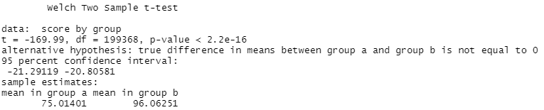
Sure enough the scores are very significantly different between groups. The scores average at around 75 in group A and 96 in group B, a mean difference of around 21. Because of how we created this data above, we already know that difference is driven by the age and height differences between groups. But an analysis as basic as that one can’t correct for that and may incorrectly conclude that whatever happened to group B participants made them get better scores. So here’s a case where matching can be an invaluable tool.
Calculating the distances between participants
The first step with quickmatch is to calculate the distances between each participant; i.e. how similar they are to each other. Small distances indicate more similarity, and hence likely closer matches. We can do that with the distances function. This function calculates the Euclidean distance between datapoints as and when needed, in a speed and memory efficient manner.
It expects numeric fields. So if you have categorical data, you should either convert it to numerical directly or make it into a factor which the function will then coerce to numeric.
Note that this is conceptually simple if you have either just 2 categories or the categories are ordinal (and specified in the factor as being so, in a logical way). If you have 3+ non-ordinal categories it may be a little more complicated.
For instance if you’ve a colour field that includes the values red, blue and yellow then it’s not clear that’s there’s any intrinsic order in terms of similarity. Is red more similar to blue or yellow? Creating a factor of this column might for instance result in red being treated as the number 1, blue as 2 and yellow as 3. The implication of this is that red is more similar and hence matchable to blue than yellow. If this doesn’t make sense in your analysis then perhaps you’d need to use a different technique or if you’re happy with only matching within a given colour – mandating that all red people should be matched with other red people and so on – you could work around this by performing 3 matches. First match only red people with each other, then blue people with each other and finally yellow people with each other before combining the results. This will be necessarily a bit suboptimal though, especially if colour isn’t the only especially important field with regards to the outcome.
In our example though we’ve got a simple 2-way categorical field “sex” here. For some of the functions later on it’s going to be useful to have an actual numeric field so let’s create instead a field “female” that’s 1 if the sex is F and 0 otherwise.
data <- mutate(data, female = if_else(sex == "F", 1, 0))
Next let’s use the distances function to create the distances object we’ll need.
library(quickmatch)

distances <- distances(data = as.data.frame(data),
                                  id_variable = "id",
                                  dist_variables = c("age", "height_cm", "female")
                                  )
Note:
- It’s important that your data is a standard R dataframe. Because of how I created my dataset it was technically a tibble object which won’t work here. But it’s easy to convert to a dataframe with the
as.data.framefunction as above. - The
id_variableparameter gives you a way to identify each of your participants. It’s optional but I find it to be useful. Here I gave it theidcolumn of my data, which I created in a way such that it’s unique per fictional participant. - The
dist_variablesare the names of the fields I want the algorithm to use when calculating distances. It’s optional – if you don’t include it it’ll use all the columns in your data except theid_variable. - There are other parameters available that can be used to normalise or weight the data. See the documentation for more on that.
Within seconds the distances object was created.
Match participants using the calculated distances
This uses the quickmatch function. The most basic call here, which we’ll use for our example is:
qm_results <- quickmatch(distances = distances, treatments = data$group)
This performs a generalised full matching. Participants are assigned to a group such that the folk within a group are as similar as possible. The distances parameter uses the distances object created above, and the treatments parameter specifies the treatment group A vs group B assignments that we’re trying to match participants between.
Every participant will be put into a matched grouping – one way to think about it is as a cluster. Some matched groups will be of different sizes to others and will contain different number of participants from each treatment group. For instance, perhaps matched group one has 1 person from treatment A and 1 from treatment B in it, whereas matched group two has 2 people from treatment A and 3 from treatment B. It simply depends on the breakdown of how similar participants are to each other.
This function is also extremely fast, taking just a couple of seconds in this example. I’ve never had to wait more than say a minute in my experimentation, compared to several hours for other matching approaches I’ve used.
There are several other optional but useful parameters you can use to further control the matches. As always the documentation explains these well. Some of them include:
treatment_constraintsandsize_constraintsthat let you specify the minimum number of people from each treatment group that should be in each matched grouping, and the minimum total number of people you want in each matched grouping.caliperwhich lets you specify a maximum distance away that you consider “good enough” for participants to be put into a matched grouping together. If you do specify this then it can be possible that some participants are just not similar enough to any potential matches to form a valid matching, in which case they’ll be discarded.targetlets you specify which treatment group you want to target, if any. It guarantees that all participants in the target group will be put into a matched grouping. Participants that are in other groups may be discarded if they’re not needed to fulfill this criteria. This is akin to calculated the average treatment effect for the treated (ATT) as opposed to the default average treatment effect (ATE). This page explains what the difference between those and several other types of treatment effects are.
Check the quality of the match results
quickmatch provides a couple of useful functions here.
covariate_balance gives you a measure of the balance between groups by calculating normalised mean differences between the treatment groups. If you specify a matching object then it will show the post-matching balance. Otherwise it shows the balance of the original unmatched data.
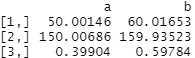
For the unmatched data you can thus do:
covariate_balance(treatments = data$group, covariates = data[c("age", "height_cm", "female")])

Note how the output values are essentially the absolute standardised mean differences we saw in our pre-matched tbl_summary output above for age, height and sex.
If you feed in the match object you created with quickmatch you’ll see the equivalent results from your treatment groups after matching, i.e. after they’ve been clustered and weighted to produce groups as similar as possible.
In this case we get:
covariate_balance(treatments = data$group, covariates = data[c("age", "height_cm", "female")], matching = qm_results)

…showing much, much lower differences between groups. None of them are near the 0.1 SMD threshold that’s typically what we worry about that we saw above.
We can also see the averages per treatment group before and after the matching exercise, this time using the covariate_averages function. It works in a similar way. If we don’t specify a matching result we get the averages from our original unmatched dataset:
covariate_averages(treatments = data$group, covariates = data[c("age", "height_cm", "female")])
Again you may recognise these figures from the tbl_summary output we produced above (albeit these are mean averages whereas I let gtsummary calculate its default medians). Group A has a lower age, height and proportion of females than group B.
If we feed in the matching object we created above, we see the averages in our now-matched dataset.
covariate_averages(treatments = data$group, covariates = data[c("age", "height_cm", "female")], matching = qm_results)
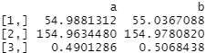
The post-matched averages between groups are far more similar. Weighted post-matched A and B treatment groups both have average ages of around 55, heights around 155cm and a roughly 50:50 split of males vs females. This is exactly what we want to see!
Both these functions have several other parameters you can use, including the target parameter discussed in the above section on the quickmatch function. In fact, to avoid continuously repeating myself, please assume that all the functions I use in my simple examples here have more parameters and functionality than I describe!
Compare the outcomes between treatment groups after matching
You can actually use covariate_averages to get the difference in outcome averages between groups by specifying whatever the outcome variable is as a covariate.
Before matching we saw:
covariate_averages(treatments = data$group, covariates = data$score)
You might remember those average score numbers from our t test results at the start. Group A has a much lower average score than group B in the raw data.
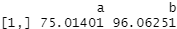
But after matching:
covariate_averages(treatments = data$group, covariates = data$score, matching = qm_results)

The average scores are extremely similar. This, as we know from how we constructed the data, is the “correct” result. The score was generated as a function of age and height plus some randomness. So once we’ve ensured groups A and B are set up to effectively have folk with the same distribution of ages and heights, the scores are likewise very similar. Our conclusion as to whether group A has different scores from group B dramatically changes.
Another way to look at the post-matching differences between treatment groups if you want obtain point and variance estimates, along with the ability to include the effects of other variables is the quickmatch lm_match function, which performs a weighted regression on the match results.
With a simple base-R linear regression we can compare the results of the raw data’s estimation of the coefficient for the impact of being in a group, calculated like this:
lm(score ~ group, data = data)$coefficients
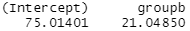
It shows a 21 point increase in score associated with being in group B.
Then we can calculate something similar for the post-matched data like this:
lm_match(outcomes = data$score, treatments = data$group, matching = qm_results)
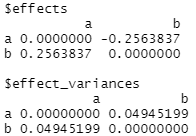
The matched sample results show a tiny 0.26 difference in scores by group assignment vs the unmatched version’s 21 points (as we’ve used simple linear regression here in both cases it’s basically the differences in mean scores between groups).
If you want to incorporate other variables into your estimation of the matched sample’s group effect you can do so in the following manner:
lm_match(outcomes = data$score, treatments = data$group, covariates = data[c("age", "height_cm", "female")], matching = qm_results)
And finally, if you want to access the actual weights of the post-matched samples themselves, perhaps in order to use in other functions, they’re available via the matching_weights function.
matching_weights(treatments = data$group, matching = qm_results)
Digging deeper into the underlying functions to perform different styles of matching
Until recently, for better or worse, I’ve typically used a different approach to creating matched groups as opposed to the weighting method this package uses. The most simple version of which was to create 1:1 matched groups. In these instances I’m typically using a smaller “treatment group” for which I want to pick similar folk from a much larger “control group”
Imagine group C consists of 100,000 people who have experienced a certain intervention and group D consists of a greater 5 million person population who haven’t. I want to end up with a set of 100,000 people from group D that are are similar as possible in terms of the distribution of specified variables to the 100,000 people in group C. I’ll then discard the remaining 4,900,000 less similar group D folk and work with two identically sized and highly matched groups from that point on. Note the obvious downside of this approach that you lose all the potential information embedded within the 900,000 discards – but then again, with samples this large that may be of less pertinence.
Thanks to the information Dr Sävje kindly provided I learned that some of the functions underlying the quickmatch package can help work with multiple groups consisting of large samples in line with this approach too. It might well be that I would be better advise to switch to the quickmatch default weighting approach, but for the sake of completeness I wanted to record some of the other possibilities here too.
1:1 matching between two treatment groups
I created a dataset with the above parameters to work with. Group C has 100k participants and group D has 5 million, but in all other respects group C resembles the definition of group A and group D resembles group B.
I now want to iterate through everyone in group C and find their nearest match in group D, and extract their IDs.
The distances function we used above actually comes from another of Dr Sävje’s R packages, itself called distances. That package also includes a nearest_neighbour_search function that can by used in this case to locate the nearest neighbour – i.e. the participant that is the shortest Euclidean distance away from the point in question – to a given set of participants.
Again we start off by creating the distances object in the same way as we did above when using quickmatch directly.
distances_2 <- distances(data = as.data.frame(data_2),
                                  id_variable = "id",
                                  dist_variables = c("age", "height_cm", "female")
                                  )
Then we can use nearest_neighbour_search to search the distance results for the nearest neighbour in group D to each participant who is in group C.
library(distances)

nns <- nearest_neighbor_search(
  distances = distances_2,
  k = 1,
  query_indices = which(data_2$group == "C"),
  search_indices = which(data_2$group == "D")
)
We feed in our distances object, and specify the other parameters such as:
kis the number of neighbours to search for. You could specify 2 for instance if you want the closest 2 participants to the one under consideration. Here I used 1 to get a 1:1 match.query_indicesis an integer vector that specifies which participants you want to search for a nearest neighbour to. In this case I specified something that translates to each participant in group C.search_indicesis a similar vector that specifies which participants to search for neighbours within; here everyone in group D.- There’s also an optional
radiusparameter if you want to restrict how near a datapoint must be to be considered a neighbour.
To extract the matches so you know which participant in D was matched with which participant in C, you can do something like this, where id was the name of the field holding the unique ID per participant I had in my original dataset.
nn_matches <- as_tibble(t(nns), rownames = "participant_id") |>
  rename(nn_index = V1) |>
  mutate(matched_id = data_2[nn_matches$nn_index, ]$id)
This results in a dataframe (well, tibble) that has the participant_id of everyone in my group C linked to their nearest match in group D (matched_id).
Note that in this case my participant IDs were actually just their row number in the original dataframe, which is why the nn_index matches the matched_id. This won’t be the case if you have some other kind of identifier for your participants.
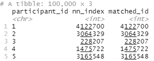
So in the above, participant_id 1 from group C was matched with participant_id 4122700 from group D.
Let’s check how well the matching went! Here I convert the above participant_id to matched_id table back into a “tall” format with 1 row for each participant. But only for the 200k participants that survived the match; half are from group C and half are from group D.
# get data into tall format
nn_matched <- bind_rows(
  select(nn_matches, id = participant_id) |>
    mutate(id = as.integer(id)),
  select(nn_matches, id = matched_id)
) |>
  left_join(data_2, by = "id")
Then we can use the gtsummary library again to check the differences before and after. Before matching that looked like this:
tbl_summary(data_2,
  by = group,
  include = c(age, height_cm, female)
) |>
  add_difference(~"smd")

As expected, big standardised differences in age, height and whether they’re female between smaller group C and larger group D.
But for the 200k matching survivors:
tbl_summary(nn_matched,
  by = group,
  include = c(age, height_cm, female)
) |>
  add_difference(~"smd")
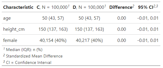
Now we have 100k participants in both groups, with extremely similar demographic breakdowns.
Note that nearest_neighbor_search treats each search for a neighbour individually, and checks against the entire possible sample you’ve asked it to find matches from. In the above, this means that the same participant from group D might be allocated to more than one of the target group C participants if that group D participant happens to be the most similar person to multiple group C folk. Essentially this is “matching with replacement”.
If re-using the same “control” person is for some reason unacceptable for your specific analysis and you’re after a matching without replacement style system then one workaround Dr Sävje mentioned was along the lines of determining the set of matches that ended up selecting a person that had already been selected for a previous match. Then re-run the matching algorithm just on those people using only the search_indices parameter for people who hadn’t yet been selected.
Repeating that enough times will eventually result in unique 1:1 matches, at the expense of them being potentially less optimal (e.g. if X matches both Y and Z, but you force Z to match something else then it might be that it’d actually have been better to keep X and Z together). This makes it more like a greedy matching algorithm. Optimal matching algorithms of course exist but are generally not performant enough for large datasets like this, at least on my computer. His advice though was that in general it is often actually statistically better to match with replacement, even if it’s less intuitive.
k:k matching between more than two treatment groups
The nearest neighbour matching described above assumes that there’s two treatment groups – one to select participants from, and another to search for neighbours within. There’s no obvious way to use the nearest_neighbor_search function directly to handle cases where you have more than two groups, contrary to the ability quickmatch has to handle unlimited groups.
As Dr Sävje describes, nearest neighbour matching group A to group B, and then group A to group C may be one hacky workaround, but does not necessarily result in good matches between group B and C. At large sample sizes this may be less of an issue though.
In any case, we can use another of his packages, scclust, which is also used within quickmatch, to cluster members from any number of treatment groups into buckets of similar participants to perform this type of exercise more reliably.
Having now created a dataset with groups E, F and G – E has 100k participants, F and G both have 2.5 million each – we can use the sc_clustering function to do the hard work here.
First create the distances object as per usual:
library(scclust)

distances_3 <- distances(
  data = as.data.frame(data_3),
  id_variable = "id",
  dist_variables = c("age", "height_cm", "female")
)
Then perform the clustering:
clustering <- sc_clustering(
  distances = distances_3,
  primary_data_points = which(data_3$group == "E"),
  type_labels = data_3$group,
  type_constraints = c("E" = 1, "F" = 1, "G" = 1)
)
- As usual we pass in the distance object to the
distancesparameter. primary_data_pointsallows us to specify a group in which it’s guaranteed all datapoints will feature in matches. It’s optional if you do not want to target a particular group, similar to how thetargetparameter works in some of the functions mentioned above.type_labelsdesignates how we’re labelling our treatment groups in the data – this field contains either E, F or G in my test dataset.type_constraintsoptionally lets us set the minimum number of participants from each group that must feature in each cluster determined. Here we’re requiring that at least one person from each group must be in each cluster.
Converting the output to a dataframe will show us which cluster (cluster_label) each participant (here id) has been assigned.
clustering |>
  as_tibble()

Anyone who didn’t get assigned a cluster, for example due to any constraints you gave that left them with no possible matches, will have an NA cluster_label.
Something like the below then will allow you to easily see which participant IDs from which groups have been assigned to each cluster. Participants with the same cluster_label should be similar to each other.
sc_clusters <- sc_clusters |>
  mutate(id = as.integer(id)) |>
  filter(!is.na(cluster_label)) |>
  left_join(select(data_3, id, group), by = "id") |>
  arrange(cluster_label, group)

One thing to notice is that whilst we guaranteed that someone from every group would be in each cluster, it’s very possible that more than one person from the same group will be in some clusters. You can see in the above example that cluster_label 1 has two group E participants, alongside one group F and one group G person. This indicates that the two group E participants are similar to each other, as well as being similar to the allocated F and G participant.
If you do require literal k:k matching, for example for the 1:1 matching example discussed above, then we will need to do something so each cluster ends up having the same number of people of each treatment group in it. Imagine for instance that if cluster 1 has two group E participants, we also want it to have two group F and two group G participants.
A ‘matching with replacement’ approach might be to establish the treatment group with the largest number of participants in each cluster. Then, within that cluster, pick at random from the participants in each other treatment groups within in the same cluster. Do that enough times such that you end up with the same number of people from each treatment group as you have in the treatment group with that has the most frequent presence in the cluster at hand.
For example, if we’d seen 3 group E people in one cluster but only 2 group F and 2 group G participants we could randomly pick 3 times from the 2 group F and G people to get enough matches for a 1:1 relationship with the 3 group E people. This, being of a “with replacement” nature, of course means you will re-use the same participants multiple times.
If “without replacement” is for some reason a requirement despite the advice above that it often produces worse results, and you don’t mind losing sample size – perhaps not a big issue with datasets will millions of entries – then another alternative could be to randomly discard the participants from the larger treatment group(s) of any cluster until you have the same number of participants from each treatment group in a cluster.
In the above example of a cluster involving 3 Es, 2Fs and 2 Gs, we would discard a group E person from the cluster such that we’re left with 2 group E, 2 group F and 2 group G participants.
Hastily-written code to do something like that might look something like:
# Calculate the smallest number of participants from any group per cluster

sc_cluster_minimum_participants_per_cluster <- sc_clusters |>
  group_by(cluster_label, group) |>
  summarise(count_of_participants = n()) |>
  group_by(cluster_label) |>
  summarise(min_group_size = min(count_of_participants))

# Now to get a 1:1 match let's select n from each cluster, where n is the minimum sample count in that cluster for any group

matched_participants <- sc_clusters |>
  left_join(sc_cluster_minimum_participants_per_cluster, by = "cluster_label") |>
  group_by(cluster_label, group) |>
  mutate(row_number = row_number()) |> # make a row count within the group
  filter(row_number <= min_group_size) |> # remove any rows that are of a larger number than the number of participants in the smallest group inside the cluster
  select(-min_group_size, -row_number) |>
  ungroup()
We can then summarise our remaining matches to check that we have the same number of participants in each group and that they are reasonably similar in terms of attributes.
matched_participants |>
  select(-group) |>
  left_join(data_3, by = "id") |>
  tbl_summary(
    by = group,
    include = c(age, height_cm, female)
  )
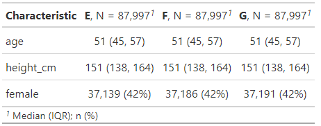
And sure enough they are! They’ve essentially the same average age, heights and propensity to be female.
Note that in following this “discard the excess participants to make each cluster have the same number of people per treatment group as the smallest treatment group within that cluster does” strategy we inevitably lose more of our participants than we would have done had we used a different approach. Our smallest treatment group in this data, E, started off with 100,000 members. As you can see from the Ns in the above table, we’ve ended up with around 88k matches; losing roughly 12% of our group E participants.

Thanks for the time you spent on this post. Well done!
Francis
LikeLike