If you’re working in R, especially in RStudio, then using the R Markdown format is a great way to organise and later render your analysis in the form of a visually pleasing and potentially interactive document.
It’s a version of the classic analysis notebook format – chunks of real working code in between explanatory text, document structure and so on; great for promoting transparent and reproducible analysis.
The non-code side of things can be formatted using markdown. Markdown is a relatively simple and readable syntax for formatting documents, originally designed to make it easy to write content for the web without knowing HTML. As far as I can tell it’s exploded in popularity. Even very non-technical products such as Slack and Google Docs allow one to use variants of markdown to some extent.
Back in the R Markdown specific world: once you’ve created the code and commentary then you can have it render to several formats – HTML, PDF, Microsoft Word, slide decks, interactive dashboards and more.
From RStudio’s introduction to the technology:
R Markdown provides an authoring framework for data science. You can use a single R Markdown file to both
- save and execute code
- generate high quality reports that can be shared with an audience
You render or “knit” the file by hitting the “Knit” button in RStudio (or manually calling the render() function from the rmarkdown library if you have a preference or need to do so) and get back a file in one of several standard formats that you can for instance share with colleagues who know nothing about R.
I find the knit-to-html workflow a great way to share reports that will likely have to be re-run in future with colleagues. If you’ve designed it considerately then when you need to update it with e.g. with new data in the future, you can just hit a button and off it goes.
Whilst it’s very simple to use in its basic form, the rendering process turns out to be a lot more sophisticated and controllable than I’d originally realised. There are several ways to control the content and style of the output. For a quick one-off render of something adhoc you may not want to spend the time fiddling with these settings. But if it’s a regular report, particularly a lengthy one, then spending some time to make it attractive and usable might be worth it.
The library that generates the output from R Markdown, Knitr, has extensive high quality documentation here that if you want to become familiar with what’s on offer in detail is well worth a read. There are several areas I haven’t dug into yet. But below are the bits that I have found myself using a few times, along with some tips and tricks picked up along the way. I have only tested this with the HTML output format, although a lot of it may apply to others.
The first thing to know is that there are at least three places that you can configure the knitted output within your R Markdown file:
- The first is at the document level. You can add parameters to the YAML metadata at the top of your R Markdown (.Rmd) file that control the rendering of the entire document. Note that YAML is very sensitive to white space and indents. If it seems like you’re not getting the result you expect then the first thing to check is that the structure is exactly correct.
- The second is at the “chunk” level. Wherever you have a chunk of R code you can use parameters to the chunk headers that will control the rendering of that particular chunk.
- The third, rarer is at the markdown header level. You can add parameters to your markdown headers that modify how the content encapsulated within the header shows up.
Now, on to more specific use cases:
- Adding a table of contents
- Themes
- Preventing certain sections of code being evaluated
- Hiding parts of the output
- Displaying content generated within functions
Adding a table of contents
At the document level, if my report is going to be quite lengthy, I often like to include a table of contents. Adding a toc: true parameter to the top of the file will automatically generate one at the top of your document.
The sections that appear in the table of contents are defined by the markdown headers in your R Markdown document. In line with standard markdown practice, top level headers start with one #, second level headers with ## and so on.
Knitr can use these headers to automatically make a table of contents whereby the user can click on a link to get to the appropriate section of the report.
There are various styles of tables you can make. You can also define how deep into the headers you want to go. For instance do you just want the top level headers showing? If so, that’s toc_depth: 1. If you would also like the second levels headers to show up, then toc_depth: 2.
For example, knitting a Rmd file that looks like this:
---
title: "Example R Markdown file"
output:
  html_document:
    toc: true
    toc_depth: 3
---

## My first header

The average MPG in the mtcars dataset is:

```{r some_r_code}
mean(mtcars$mpg)
```

### My second header

More example text.

## Another header

Last bit of text
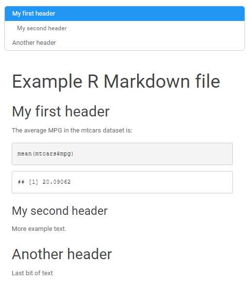
Gives you output that looks like:
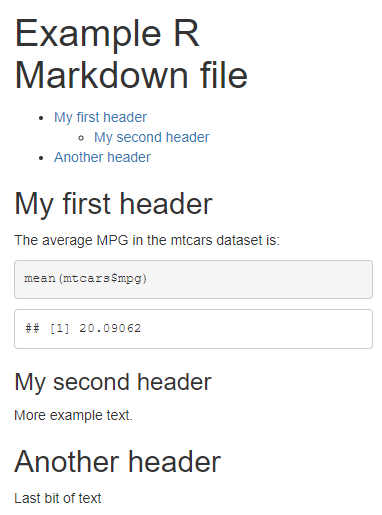
The links shown just under the “Example R Markdown file” title are the table of contents. Clicking those links scrolls the document to the appropriate header.
I personally prefer a floating table of contents style, especially for a long document. It allows users to see and navigate through the structure of your report even when they scroll far down into it. Add the toc_float: true parameter if you want this. In that case the header of your document would look like:
title: "Example R Markdown file"
output:
  html_document:
    toc: true
    toc_float:
      collapsed: false
    toc_depth: 3
And the rendered output would look like this:
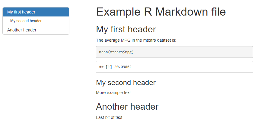
Using this style, the table of contents appears on the left of the browser window and stays at the top when you scroll down through the contents of the document. On one as short as this that’s not super useful. But on longer reports with many sections, it’s great to have a way for the user to flick between sections quickly. Another good feature is that the section of the report the user is reading is highlighted in the table of contents, giving the user a sense of where they are and what they’re looking at.
You can also choose to have the hierarchy of headers expanded or collapsed by default. That’s what the collapsed parameter controls in the above code – true or false. If false, only the top level headers are shown by default. The user can click on them to make their sub-headings visible.
Note that if the browser window isn’t wide enough, for instance if someone is using a phone to read your report, then the table of contents will appear at the top of the report, not visible when the user scrolls down.
Behind the scenes, this floating version is using a jQuery plugin called tocify, which might be useful information if you’re looking to customise it in a more advanced way.
If you have certain markdown headers that you’d rather didn’t feature in the table of contents, you can add parameters inside curly brackets right after the header to control that.
If the “Another header” text was set to be unlisted and toc-ignored like this:
## Another header {.unlisted .toc-ignore}

Last bit of text
Then when knitted the “Another header” header will still appear in the document, but won’t be shown in the table of contents.
In theory you only need the .toc-ignore parameter if you’re rendering to the floating style of the table of contents. The default table of contents style respects the .unlisted parameter just fine.
There’s also a similar .unnumbered parameter you can add to specific markdown headings in the same way if you set your section headings to be automatically numbered but want to skip numbering the header in question. If you do want the automatic numbering to take place in general, then in the YAML header you want to set number_sections to true, something like this:
title: "Example R Markdown file"
output:
  html_document:
    toc: true
    number_sections: true
Themes
Continuing with the subject of different styles, knitr has a whole theming system built into it. To select a theme, you use the theme parameter within the YAML document header.
Currently, I quite like the “Paper” theme for my longer reports. If I wanted to make the above report use the Paper theme then I could use a YAML header like this at the top of my markdown file:
title: "Example R Markdown file"
output:
  html_document:
    toc: true
    toc_float:
      collapsed: false
    toc_depth: 3
    theme: paper
Note the theme: parameter at the bottom of that snippet.
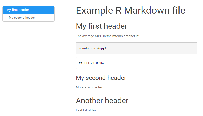
When the document is rendered I get a slightly different set of colours and fonts:
These themes are based on Bootstrap themes – if you want to see what the options are and what they look like without trying them all out yourself then they’re shown at Bootswatch.
Extra R Markdown themes can also be included in R packages. I haven’t looked into any of them very thoroughly yet but some packages that seem relevant include:
- prettydoc: “Creating tiny yet beautiful documents and vignettes from R Markdown.”
- rmdformats: “HTML formats and templates for ‘rmarkdown’ documents, with some extra features such as automatic table of contents, lightboxed figures, dynamic crosstab helper.”
- hrbrthemes has one called ipsum even though the package is mainly targeted at ggplot2 theming.
- tufte: “Provides R Markdown output formats to use Tufte styles for PDF and HTML output.”
- tint: “A modern take on the ‘Tufte’ design for pdf and html vignettes.”
- cleanrmd:” A collection of clean ‘R Markdown’ HTML document templates using classy-looking classless CSS styles”
I’m sure there are others.
If you don’t like any of them, then you can naturally create your own theme. If you know or are prepared to learn some CSS, then you can also apply custom CSS to what is already there by linking to an external style sheet or embedding it directly in your R markdown document. The R Markdown Cookbook has instructions of how to do that (and an absolute bucket-load of other customisations).
Preventing certain sections of code being evaluated
When you knit a document, it runs all the code in order, top to bottom. This is usually what you want, plus is a good way to ensure your work is reproducible. But sometimes whilst you’re iterating through the analysis you might want to be able to knit it to test what it looks like without evaluating some of the less interesting or slow-to-process sections.
This is easy to do with the eval parameter of the relevant chunk headers. Setting eval to false stops the chunk from being evaluated. It defaults to true, so if you don’t have an eval parameter at all then the code will be evaluated. Here’s an example:
---
title: "Example R Markdown file"
output:
  html_document
---

## My first header

```{r first_code}
mean(mtcars$mpg)
```


### My second header

```{r second_code, eval = FALSE}
mean(mtcars$cyl)
```

### My third header
This renders as:
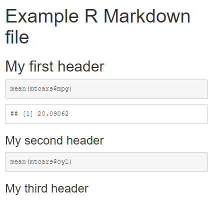
The output from this example shows that the code after the first header is evaluated, with the result of the calculation being shown in the document as 20.09062. But whilst the code of the second section is displayed, it doesn’t actually show the numerical result because it was never evaluated.
Hiding parts of the output
By default your knitted output will usually contain all the code, results, R warnings and messages that you’d see if you were to run the code in the standard interactive way, alongside the render of the markdown structure and other text in the document.
Oftentimes this is great – full transparency, and if something fails unexpectedly you’ll see it! But if you are making a report for other people to read then it can start to look messy, cluttered and hard to navigate, especially if they’re not R users used to seeing reams of R messages, some of which can look more scary than they are. If this is your use-case, then once you are confident everything is working as intended analysis-wise you might want to prevent any interim results, warnings and messages being displayed.
Stopping the entire chunk being evaluated as described above is one way to stop its output showing up. But if you need the chunk to run to provide input to later chunks then setting eval to false will break your work. Even if you can safely skip evaluation of a chunk the skipped code is still shown in the output by default which might not be what you want.
Luckily there are various options you can set in the relevant chunk header that will still allow the chunk to be evaluated behind the scenes but hide some or all of the visible output it would by default produce in the rendered file. Simply add X = false to the chunk header, where X is one of:
error: if you want to hide errors.warning: if you want to hide warnings.message: if you want to hide messages.echo: if you want to hide the code.
You can add several of these to the same chunk to get the combined effect.
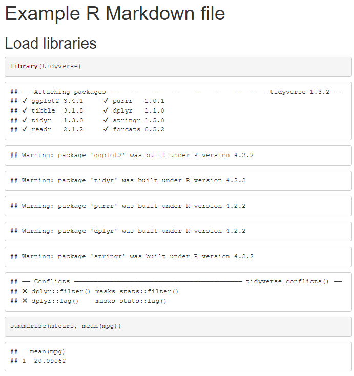
For example, just loading and calculating an average using the tidyverse library results in an array of messages that end-users might not care about when knitted:
---
title: "Example R Markdown file"
output:
  html_document
---

## Load libraries

```{r libraries}
library(tidyverse)
summarise(mtcars, mean(mpg))
```
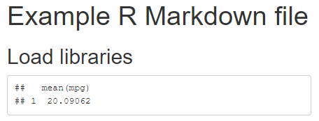
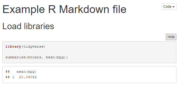
Adding warning = FALSE, message = FALSE, echo = FALSE to the chunk that loads the library and summarises the data like this makes for a much cleaner output:
```{r libraries, warning = FALSE, message = FALSE, echo = FALSE}
library(tidyverse)
summarise(mtcars, mean(mpg))
```
Of course this means that when you run the file it will never show you any warnings, so you’d want to be confident your code works properly before enabling this feature!
Another option you have if you want to hide code by default but still allow users to choose to see it if they want is to add a code_folding: hide parameter to the YAML at the top of your file, in this manner:
title: "Example R Markdown file"
output:
  html_document:
    code_folding: hide
With that, the R code driving your analysis will be hidden, but each section where code would have been has a “Show” button. If the end-user wants to, they can hit “Show” and the code will drop down to make it visible to them. You can also set code_folding to true if you want the ability to show or hide the code but prefer it to be shown by default.
That would look something like this – note the “Hide” button to the top right of the code. If the user presses that the code will fold away, with the button replaced by a “Show” button to enable it to be re-shown if desired:
Outside of code chunks, you can stop whole sections of your markdown documents being rendered when knitted without having to remove the text from the .Rmd file itself. This can be useful if you leave extensive notes-to-self-and-other-analysts in them as I do but don’t want them all displayed to the average end user of the report.
To do this, you can place .hidden in curly braces right after the relevant markdown header.
With markdown that looks like this:
---
title: "Example R Markdown file"
output:
  html_document
---

## Load libraries
  ```{r libraries, warning = FALSE, message = FALSE, echo = FALSE}
library(tidyverse)
```
## Do calculations {.hidden }
```{r calculation}
a <- 2 + 2
```

## Show results
```{r show_result}
a
```
You get the following result when knitted:
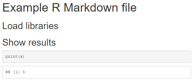
Notice how because we added the {.hidden } attribute to the “Do calculations” header, neither the header itself or the subsequent text or code chunk are shown. But we can see that the code was still evaluated behind the scenes, as the “Show results” section displays the appropriate answer.
Displaying content generated within functions
Writing custom R functions is often invaluable, particularly in large reports that would otherwise require repetitive code. However, if the purpose of the functions is to add some visible content to the rendered output then one has to take a little care to make that explicit. By default the interim results of code held within a function will not show up. How to make them do so depends on the nature of the content you’re trying to display.
To see an example of why this is a problem, consider the following file:
---
title: "Example R Markdown file"
output:
  html_document
---

## Load libraries

```{r libraries, warning = FALSE, message = FALSE, echo = FALSE}
library(tidyverse)
library(gtsummary)
library(plotly)
```

## Define a function that produces output

```{r function_def, echo = FALSE}

show_output <- function() {
    2 + 2

    ggplot(mtcars, aes(x = factor(cyl))) +
      geom_bar()

      # Show a HTML gtsummary table
    tbl_summary(mtcars,
      by = "cyl",
      include = c("mpg", "disp", "hp")
    )

  # Show an interactive HTML chart
      ggplotly(
        ggplot(mtcars, aes(x = factor(cyl))) +
          geom_bar()
      )

  # return something as an example
  return(pi)
}
```

## Show output

```{r show_output, echo = FALSE}

# Run the functions
show_output()
```
I defined a show_output() function that produces the result of a sum (2+2), a chart and a HTML summary table as created by the gtsummary library and an interactive HTML and JavaScript chart created by the plotly library. This function is then called at the bottom of my markdown file, in the “Show output” header section.
When I knit this I get the following:
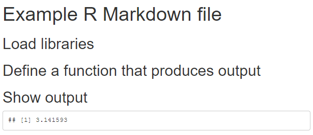
No sum, chart, table or chart! The only thing that is displayed in the rendered output when the show_output() function is called by the “Show output” section is the return value of the function; in this case the value of pi.
But what if you wanted to see the intermediate output of the function? i.e. the text, charts and HTML output that would have appeared had you called them directly, rather than in a function.
One alternative would be to have your function return a list of whatever is to be displayed and separately show it once you’re back outside of the function. That might be “purer” in a sense. But sometimes it’s just easier or more code-efficient to have the function itself show the output. What you need to do to enable this depends on the type of content you’re trying to render.
Text and images
If it’s just pure text or a basic image then it’s easy. You just enclose it within the print() function. Surround the relevant bits of code within the function like this and their results will show up in the output:
show_output <- function() {

  # show the results of a sum

  print(2 + 2)

  # Show a ggplot chart
  print(
  ggplot(mtcars, aes(x = cyl)) +
    geom_histogram()
  )
}
Basic HTML
If what you’re trying to display is actually HTML content, then calling print() on it prints out the HTML code itself, not what the HTML would be rendered into in a standard browser. In the example above where I tried to use the tbl_summary function I get reams of code like the below in my post-knit file.
## <div id="fnnhhegzmh" style="overflow-x:auto;overflow-y:auto;width:auto;height:auto;">
##   <style>html {
##   font-family: -apple-system, BlinkMacSystemFont, 'Segoe UI', Roboto, Oxygen, Ubuntu, Cantarell, 'Helvetica Neue', 'Fira Sans', 'Droid Sans', Arial, sans-serif;
## }
##
## #fnnhhegzmh .gt_table {
##   display: table;
##   border-collapse: collapse;
The two hashes you see to the left of each line are part of what’s causing the problem here. They reflect how you use comments in R. But if you want to render the HTML generated by the tblsummary function here rather than an R-sanitised version of the code behind them then they’re unhelpful.
The solution is to use the chunk option {results = "asis"} to tell the rendering engine to simply accept the output as is, and not to try and do anything “clever” such as wrapping it in comments. Do this in the code block that calls the function and is thus in charge of the display of whatever the called function produced, not the chunk that defines the function itself.
This is the relevant snippet you’d want want in my above example:
## Show output

```{r show_output, results = "asis"}
show_output()
```
HTML with Javascript (e.g. DT , gt, plotly)
Some libraries output HTML widgets that allow a degree of user interactivity via JavaScript, These include gt and any of its derivative that use it such as gtsummary, plotly, the datatables from the DT library and many more.
If you just put the "asis" and print() in place as detailed above you still won’t see these type of interactive widgets rendered. The reason why seems (to me) to be quite complicated, but there is at least a solution that reliably works. That’s to wrap the Javascript-generating function up in another function, tagList, from the htmltools library.
This is what would work for the attempt at outputing an interactive plotly chart in the above example:
show_output <- function() {

# Show an interactive HTML chart

  print(
    htmltools::tagList(
      ggplotly(
        ggplot(mtcars, aes(x = factor(cyl))) +
          geom_bar()
      )
    )
  )
}
One final trick may be needed. If the JavaScript engine hasn’t been initialised anywhere outside of the function in your script (for example by a previous portion of your script rendering some JavaScripty output outside of the function) then you may just get a blank white box in your output when you print(taglist(...)).
The most relevant discussion about this I could find is probably this one. All in all, it doesn’t sound like it’s exactly a “bug” but it definitely requires you to work around it.
The workaround in question is to initialise the JavaScript engine outside before you call your function. For example you could do it in the chunk where that call the function from. To do this you basically want it to try and render something of that type once, and then all future renders in your file should work.
Of course ideally you don’t want unnecessary clutter in your markdown output. Borrowing examples from the conversation mentioned above and elsewhere you can initialise the engine without showing any visible output in your rendered file by running something like:
htmltools::tagList(plotly::ggplotly(ggplot())) |>
  knitr::knit_print() |>
  attr('knit_meta') |>
  knitr::knit_meta_add() |>
  invisible()
That example uses a function from the plotly library. If instead you’re using the DT library then there’s no need to install plotly just for the sake of this. Instead, something like this would work:
 data.frame() |>
   DT::datatable() |>
   knitr::knit_print() |>
   attr('knit_meta') |>
   knitr::knit_meta_add() |>
   invisible()
You can probably see the pattern. It should work with any library that has this kind of output. Just make sure it runs in your file before you call your function.
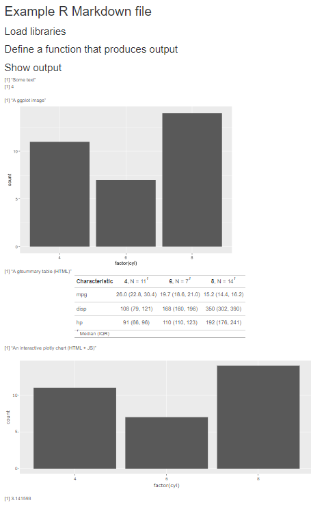
All in all, the below file shows how to visibly render a mix of text, images, HTML and HTML + Javascript that all reside within a function.
---
title: "Example R Markdown file"
output:
  html_document

---

## Load libraries

```{r libraries, warning = FALSE, message = FALSE, echo = FALSE}
library(tidyverse)
library(gtsummary)
library(plotly)
library(htmltools)
```

## Define a function that produces output

```{r function_def, echo = FALSE}

show_output <- function() {

  # show some text
  print("Some text")
  cat("<br />") # <br /> is the HTML for a linebreak, this is just for formatting.
  print(2 + 2)
  cat("<br />")
  cat("<br />")


  # Show a ggplot chart
  print("A ggplot image")
  cat("<br />")

  print(
    ggplot(mtcars, aes(x = factor(cyl))) +
      geom_bar()
  )

  # Show a HTML gtsummary table
  cat("<br />")
  print("A gtsummary table (HTML)")
  cat("<br />")
  print(
    tbl_summary(mtcars,
      by = "cyl",
      include = c("mpg", "disp", "hp")
    )
  )

  # Show an interactive HTML chart
  cat("<br />")
  print("An interactive plotly chart (HTML + JS)")
  cat("<br />")
  print(
    htmltools::tagList(
      ggplotly(
        ggplot(mtcars, aes(x = factor(cyl))) +
          geom_bar()
      )
    )
  )


  # return something as an example
  return(pi)
}
```


## Show output

```{r show_output, echo = FALSE, results = "asis"}

# Initialise the Javascript. No need to do this if you already have done so previously outside of a function.

htmltools::tagList(ggplotly(ggplot())) |>
  knitr::knit_print() |>
  attr('knit_meta') |>
  knitr::knit_meta_add() |>
  invisible()

# Run the functions

show_output()
```
Running that gets you output like the below. The version shown here in the post is just an image. but the chart at the bottom of the actual file the code above produces is interactive, courtesy of ggplotly.