In the classic randomised experiment we randomly assign participants to at least two groups, test and control, by metaphorically tossing a coin to allocate them to one or the other. However, in reality sometimes slightly more sophisticated methods can be useful.
One such method is blocking. Here, you first create “blocks” of participants, usually based on their similarity to each other. You then select participants by randomising within each block. So perhaps you pre-filter all your female participants into one block and all your males into another. Then you randomly select 100 people from each of those blocks into both your test and control group, getting you 400 participants in total.
Why so? Well, perhaps you think that the outcome you’re testing for may be affected by the sex of the participant, but your research question isn’t trying to tackle that particular topic. In this scenario, sex isn’t not the source of variation that you’re most interested in. So you’d rather eliminate any effect that differences in sex between your groups could cause in your observations in order to gain a better idea of the effect of the intervention itself; removing a so-called “nuisance variable“.
After all, under basic randomisation, it’d be possible – albeit extremely unlikely – for you to end up with all your females in one group and all your males in another. A blocking design as described above would eliminate that possibility, and help ensure your samples are balanced by sex.
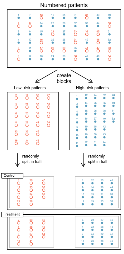
Here’s a diagram from the wonderful OpenIntro Statistics textbook, illustrating the concept in terms of blocking patients based on whether they’re deemed to be high or low risk for the medical intervention at hand. If we didn’t take this step, we’d be taking the risk that our test group may end up with a higher or lower proportion of high-risk folk than the control group has. This might be extra the case if you’re operating at the lower limit of sample size requirements, where the law of large numbers is less likely to save you.
The key requirement here is you start by creating groups of “similar” participants. One may also be able to imagine other reasons, unrelated to blocking experiments, why you might want to be able to group simliar things. But, beyond the case of a single categorical variable such as sex or risk level, how should we decide which participants are “similar” in the first place?
“Block what you can, randomise what you cannot.”
George Box (probably), source.
The actual variables you select will be specific to your experiment. The basic idea is that you want to use any factors that there’s reason to believe may confound the results of your experiment, i.e. what you want to control for. It could be sex, or it might be height, weight, income, how many blog posts someone read a day, or an infinite number of other things. So this post can’t really help you in terms of knowing which variables to consider.
But once you’ve selected those variables, the next question is how should we use them to determine which participants are most similar to each other, multi-dimensionally if needed, and hence the definition of the blocks you should randomise from. And here’s where this post, or more accurately, Ryan T. Moore and Keith Schnakenberg, the authors of the R package, “blocktools“, can help.
Let’s test it out with the following contrived, and unrealistically small, dataset. Imagine we have 10 – I did say unrealistically small, remember – potential participants we want to allocate equally to test and control groups in order to test the effects of some intervention on them. In terms of pre-existing information, we know their age, their score on some test, their height and their current location.
| participant | age | score | height | location |
| A | 3 | 3 | 50 | New York |
| B | 6 | 2 | 70 | New York |
| C | 8 | 2 | 80 | London |
| D | 30 | 5 | 178 | London |
| E | 40 | 6 | 175 | London |
| F | 10 | 3 | 60 | New York |
| G | 75 | 7 | 140 | New York |
| H | 80 | 9 | 145 | New York |
| I | 85 | 8 | 150 | London |
| J | 90 | 9 | 147 | London |
If we performed simple randomisation into 2 groups – a test group and a control group – then perhaps by incredible coincidence we’d end up with the the people from rows 1-5 in our test group and the folk from rows 6-10 in our control group.
Also let’s assume that we think the results of our intervention could be affected by the participant’s age, score and height.
Did our randomisation set us up for success by producing two similar groups? There’s many ways to think about answering that, but let’s take an extraordinarily simplistic one and just look at the average of those variables in each group. In R, we could calculate that in the below manner, where “data” is the dataframe with the table of data shown above in, and my_group is a column we added showing either 1 if we put the person in the test group or 2 if they’re in the control group.
library(tidyverse)

group_by(data, my_group) %>%
  summarise(participant_count = n(), across(c(2, 3, 4), mean))
The output:
| my_group | participant_count | age | score | height |
| 1 | 5 | 17.4 | 3.6 | 111 |
| 2 | 5 | 68 | 7.2 | 128 |
Let’s imagine we know already that younger, shorter people with low scores always tend to fare better on whatever we’re testing as the result of our experiment. Even if our intervention has no real effect, it might look like our test group, group 1, did indeed do better than our control group. Oh no, faulty conclusion alert!
Blocking your sample with the blockTools package
To reduce this possibility, we can use the blockTools library to block on age, score and height. Essentially we aim to produce pairs of people that are “similar” on those variables. Next, we randomise by picking one person from each pair for our test group and use the other in our control group. Doing this, we stand a better chance of ending up with two groups that are similar on those variables.
To proceed:
library(blockTools)
library(nbpMatching) # needed if you want to use the optimal matching option of blockTools

# create blocks
blocks <- block(data,
                n.tr = 2,
                algorithm = "optimal",
                distance = "mahalanobis",
                id.vars = "participant_id",
                block.vars = c("age", "score", "height")
)
Here I chose to create the “blocks” object to store my block details. To explain some of the options of the block() function:
- The first parameter, data, is simply the name of my dataframe containing the table shown above.
- n.tr: how many conditions you want per block. Here I wanted to generate a test group and a control group, so that’s 2 conditions. But maybe you want 3 similar groups (2 interventions and a control?), in which case set the n.tr parameter to 3.
- algorithm: how you want it to approach comparing the participants to determine similarity. The option I picked here, optimal, goes through and figures out the set of blocks that minimises the sum of distances in all blocks. That’s nice, but also computationally intensive so potentially slower or memory-destroying in larger datasets. It’s also only implemented for the case where you want 2 groups, i.e. n.tr = 2. Another option I’ve used here in circumstances where those limitations won’t work for me is “optGreedy”, a greedy algorithm. This one figures out the best match for the first person, and then goes down the list repeatedly finding the best match in the dataset that hasn’t already been used, until everyone has a match. This is faster and easier, but may risk the last few matches not being all that similar if all the closer matches were already allocated. Note also that if you do want to use the “optimal” algorithm then you may need to install and load the nbpMatching package.
- distance: how are we going to calculate the “distance” between each participant? Smaller distances imply more similar participants; hence the reference in the above paragraph to minimising the sum of distances. But there’s more than one way to decide whether someone with a set of values for age, score and height is more or less similar to person A who may differ mostly on age, vs person B who differs more on height. Here I’ve picked to use the default, the Mahalanobis distance.
- id.vars: the column that provides the ID of the participant. This is useful to connect the block allocations back up to your participant data later. Here’s it’s my table’s “participant_id” column.
- block.vars: the all-important information as to which columns contain the variables I want to block on. Here I chose age, score and height. These should be numeric variables. We’ll see later how you can incorporate information from a categorical variable.
There are many more parameters you can feed into the block function. For a full list you can naturally read the manual.
Once I’ve run the above blocks command, I can then just print out the values of “blocks”. This gives a quick summary of which participant was twinned up with which other one, as well as the calculated distance between the two. Lower distances would imply greater similarity, which can give you an idea of which matches may be better than which other ones in terms of similarity.
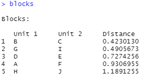
The first, closest, match here was made between participant B and participant C. They have an age of 6 and 8 years respectively, a score of exactly 2 and a height difference of only 10 cm. These people do indeed seem pretty similar, considering the options!
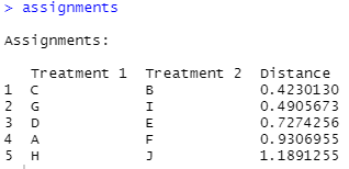
Once you have the blocks, it’s time to randomly allocate from them to form the test and control group, or however many groups you requested via the n.tr parameter above. For this, blockTools provides the assignment function. Just pass in the block object generated above:
assignments <- assignment(blocks)
Each time you run it, it randomly assigns the blocked individuals to groups. This means you’ll likely get two different allocations if you run it twice. If you want something reproducible, you can set a random seed via the seed parameter of the assignment function to ensure you get the same result each time.
The output you get when you print the assignments object looks similar to the original blocks object. But note that the headers are telling you which participants are to be in treatment group 1 and treatment group 2, rather than how the units were blocked.
For me, the next step is often to pivot the assignments result into a longer table, where I have a column per participant_id, alongside that participant’s allocation to test group 1 vs group 2 as another field in the same table. This makes it easy to integrate the group assignment back onto your original dataset if you like. Here’s one way to perform the pivot using the pivot_longer() function in from the tidyr package.
assignments_table <- assignments[["assg"]][["1"]] %>%
  pivot_longer(cols = starts_with("treatment"), names_to = "test_group", values_to = "participant_id")
That gives you an “assignments_table” dataframe that looks like this:

…which you can use directly, or perhaps join back onto your original dataframe of participant data, based on the participant_id column, like this:
data <- data %>%
  left_join(assignments_table, by = c("participant_id" = "participant_id"))
OK, so how well did our blocking-and-allocating work in terms of ending up with a test and control group with similar means in the variables we care about?
This was the summary of means per group we saw above when I just let normal randomisation run amok within my small data table:
| my_group | participant_count | age | score | height |
| 1 | 5 | 17.4 | 3.6 | 111 |
| 2 | 5 | 68 | 7.2 | 128 |
And here’s the same table, but this time using the grouping suggested by the blockTools blocking and assignment method above.
| test_group | participant_count | age | score | height |
| Treatment 1 | 5 | 39.2 | 5.2 | 119 |
| Treatment 2 | 5 | 46.2 | 5.6 | 120 |
Yep, that seemed to work quite well! We have much more similar average ages, scores and heights in our two groups; not bad at all given the contrived and tiny sample.
Adding fixed limits as to what can be considered “similar”
There are many more potential options available with the blockTools block function. We won’t go into them all here – but just a couple more before I stop.
Perhaps there’s a certain variable that’s so important to your outcome that you don’t necessarily just want “as similar as possible” matches in the manner that the above method produces, but rather than you want to introduce a hard threshold on how similar they have to be.
Here for instance, imagine that you want to insist that, no matter what else is the case, the participants that are matched together as being similar must not differ by more than five years of age.
For that, we can use the valid.var and valid.range parameters of the block function. In this example, we’re letting the algorithm know that it should only match up participants where the difference in age is between 0 and 5 years. Note that here I’ve switched to the “optGreedy” algorithm, as the valid_var functionality isn’t available if using the “optimal” algorithm.
blocks_2 <- block(data,
                n.tr = 2,
                algorithm = "optGreedy",
                distance = "mahalanobis",
                id.vars = "participant_id",
                block.vars = c("age", "score", "height"),
                valid.var = "age",
                valid.range = c(0, 5)
What do we see when we examine the block_2 object the above produced?

The algorithm managed to match up participant C with B, J with I, and H with G. However, the remaining folk couldn’t be matched so are in their own rows, with a NA, aka missing, match.
That’s because, if we look at participant A, they have an age of 3. The only participants with an age of no more than 5 years away from 3 years old are B and C. But they’ve already been matched to each other, so can’t be reused. This means there’s no further participants that fit the constraint that the ages must be within 5 years of each other. Ergo, no match can be made. You might end up taking this person out of your analysis if this sort of situation occurs in the real world and you aren’t comfortable relaxing the constraints, although you then lower the information available for analysis, and likely the generalisability of any conclusion.
If however you’re happy with the results, you can go on and use the assignment() function on the output of this call to block, as shown earlier, to assign your participants to groups.
Incorporating categorical variables
Perhaps you only want to block-and-randomise within a certain category of participant.
In our data here we had a “location” field that denoted whether the participant was currently in New York or London. Perhaps we don’t want New York people to be matched with London people; the city itself being a potential confounding factor for our imaginary intervention. To constrain the block function to only match from within specific groups of participants we can use the groups parameter.
blocks_3 <- block(data,
                n.tr = 2,
                algorithm = "optimal",
                groups = "location",
                distance = "mahalanobis",
                id.vars = "participant_id",
                block.vars = c("age", "score", "height")
Let’s see what we now have in blocks_3:

Now the output shows us that units were matched only within each location group, as specified. D and E got matched from our London residents, as did I and J. Similarly, A, F, B and G from New York all got matched up. However, we’re left with C from London and H from New York. As we specified that we only want to match folk up within each location there is no match left for these participants. Thus they are returned with a missing, NA, match.
