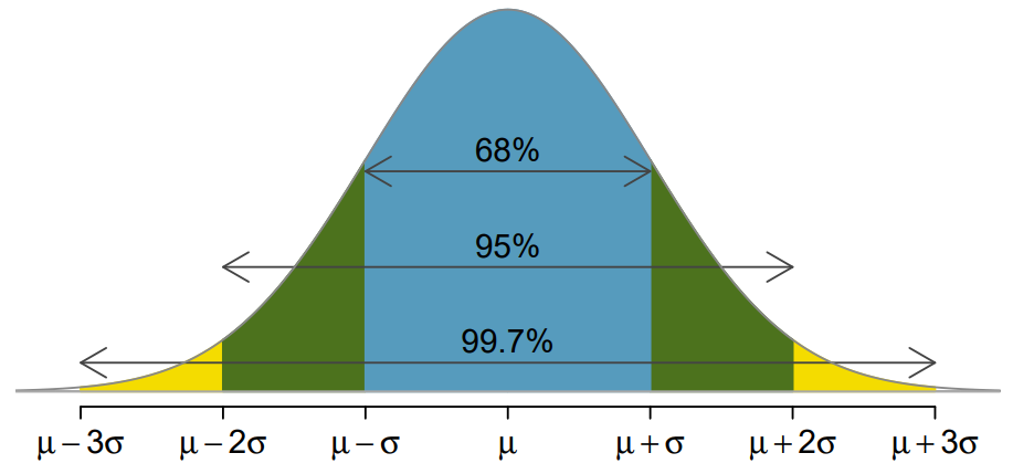
Most people that have studied a certain amount of statistics theory will likely have encountered the 68-95-99.7 rule. It could surely do with a more catchy name, but the point of it is to quickly express the proportion of values that should lie within 1, 2 and 3 standard deviations of the mean for a variable that has a normal distribution.
The OpenIntro Statistics textbook provides the classic illustration of what that looks like visually.
As an example of why this rule can be useful, let’s note that human height is fairly normally distributed. According to an Our World In Data article, the mean average height of a woman in areas where they had data was 164.7cm, with a standard deviation of 7.07cm.
Assuming we are happy to take the population as indeed being normally distributed, if we want to design a height-dependent product that will work for 95% of women then we can quickly calculate what heights we need to accommodate without any further complex math or sampling.
The “95” in the 68-95-99.7 rule is the proportion of the population that would be within 2 standard deviations of the mean, so we should ensure we design for heights between 164.7 – (2 * 7.07) and 164+ (2 * 7.07), i.e. 150.6 cm to 178.1 cm.
This formula works for any normal distribution, but only for normal distributions. In the day-to-day life of many analysts, we may be dealing with data we either know isn’t normally distributed, or we don’t have a clue what the distribution is at this point in time.
No need to despair: there’s a lesser-known alternative that provides a guideline for data from (nearly) any distribution – Chebyshev’s inequality, which you can calculate as long as you know the mean and standard deviation of the data in question. It’s of a similar form, letting us say that no more than X% of the data would likely by more than Y standard deviations away from the mean.
Here we go:
The proportion of observations that will reside within k standard deviations from the mean will be at least 1 – (1 / k2)).
So let’s try it out for 1, 2 and 3 standard deviations in order to get something to compare to the 68, 95 and 99.7% values drilled into us as being applicable to the normal distribution.
If k = 1, then the proportion of observations that will reside within 1 standard deviation from the mean will be at least:
1 - (1/(1^2))
= 0%
So we can say that at least 0% of your data from your unknown distribution will likely be within 1 standard deviation of the mean. “At least 0%” of course is synonymous with “could actually be anything” so this isn’t a particularly useful result. Which makes the point that this approach should not be applied to ranges of 1 standard deviation or below.
More usefully, when k = 2:
 1 - (1 / 2^2))
 = 0.75
So we can say that at least 75% of your observations likely reside within 2 standard deviations of the mean. The value for k = 3 works out to be around 89%.
Another way to express “at least 89% of your observations will be within 3 standard deviations of the mean” is “no more than 11% of your observations should be outside 3 standard deviations of the mean”, should you be trying to figure out how unusual something you just saw probably is.
Whilst the Chebyshev’s inequality approach is self-evidently more flexible than the 68-95-99.7 rule in that it be used with almost any distribution, that very lack of being able to assume a certain distribution means that it necessarily produces less certain, wider, intervals.
If we think again about the example above where we were interested in calculating the width of the interval that we would expect 95% of women’s heights from the population studied to be within, we determined using the “95” rule that it would be between 150.6 cm and 178.1 cm.
But what if we didn’t know, or didn’t want to assume, that height is usually roughly normally distributed? To figure out what our expectations should be around the range we need to capture to include around 95% of the population, we first need to ask what value of k would be needed in Chebyshev’s inequality to produce a “proportion of observations residing within k standard deviations” of around 0.95,
With a bit of substituting and rearranging we can do something like:
0.95 =  1 - (1 / k^2))
1 / k^2 = 0.05
1 = 0.05 (k ^ 2)
k ^ 2 = 20
k = sqrt(20) = ~4.5
…to get to a k of around 4.5. This means we can say that, without having a clue of which distribution is involved, that we should capture at least 95% of the relevant population if we look for women within 4.5 standard deviations of the mean. That would translate to thresholds of between 164.7 – (4.5 * 7.07) and 164+ (4.5 * 7.07), which works out to a range of 132.9 through to 195.8.
This is a substantially wider range than the one that the 68-95-99.7 rule implied – we’re losing quite some precision by being unable to make assumptions about the distribution. So if you know your data is normal then by all means forget Chebyshev!
Chebyshev’s formula is still perfectly valid when applied to normal distributions, in the sense that it’s both true that:
- Around 95% of the women’s heights would be between 150.6 cm and 178.1; and
- At least 95% of women have a height between 132.9 and 195.8cm
But, given a choice, there’s no reason not to use the more precise estimate given in the first point above.
However for situations where you aren’t able to live in the statistician’s dream world where Everything Is Normal, Chebyshev’s inequality will help you get a safer, more realistic idea of the likely range your data may show.
As a bonus fun fact for getting to the end of this article: it turns out that there’s a crater on the moon named after the same Chebyshev.
