Most data folk I know love experiments. They’re the ideal way to use data to answer the question of not only whether A is associated with B, but also if A causes B. Randomised Controlled Trials are a subset of experiments that most interested people seem to agree are the gold standard in, for instance, drug trials. At least if they’re designed and carried out well, and can be replicated.
But well-designed experiments usually take time and money. One reason for this is that most often you’re sampling something and, all other things being equal, the bigger sample you use the more reliable your results will be. Of course you should have done a sample size calculation to figure out what the minimum sample size is that you need to test if you want to stand a fair chance of seeing your expected effect. But usually the more people or things you have to test the more resources you need to deal with them, in terms of time, money or other real-world obstacles.
So there’s often a temptation – perhaps especially in the business world? – to check the results a bit early. After all, sure, your sample size calculation may have suggested you need to test 1000 people, but maybe your world-beating innovation is actually so great that you’ll see the effects clearly once you’ve tested the first 100 folk. So why not take a look a bit early, and if you do already see the effect you were anticipating then stop the test in order to avoid wasting resources measuring the rest, when you already saw the answer?
In the real world, when frequentist statistics are in play, this often translates to the experimenters checking in before the end of the experiment and doing a statistical hypothesis test with the data collected so far. If they see that the current dataset would imply a p value below their chosen threshold – often using the classic albeit mostly arbitrary threshold of 0.05 – the temptation is to stop there and celebrate that their experiment showed whatever they tested worked in practice.
Very cool, very fun, go home early, save big bucks, use the other 900 recruits in another experiment, whatever! What’s the harm in that?
The problem with peeking at the results of an experiment too often
Well, the harm is that you may be dramatically increasing the chances that your tremendous success is in fact a false positive.
The intuition here is similar to that which surrounds all such thorny “multiple comparison tests“. Hypothesis tests such as the t test, ANOVA et al are designed to control the false positive rate, aka type 1 errors. That’s the type of error where you think you saw an effect of your intervention on the group concerned even though in reality there wasn’t one. You claim your drug worked because more people were cured in the group who had access to it than those who didn’t, but unfortunately that was just down to random chance and it actually has no useful effect.
When sampling, one can never be 100% sure that what we see will be true for the entire population. And thus we settle for accepting a known risk of being wrong. For the “incorrectly conclude there is a real difference” category of error that corresponds to the alpha value. This value is traditionally set at 0.05, at least in the social sciences amongst other fields. Simplistically, if we set our threshold for significance at p <= 0.05, we’re roughly saying that we will conclude that our intervention had an effect if there’s no more than a 5% chance that we would have seen the same or more extreme differences between groups if in fact the intervention in fact had no effect. There’s still an unavoidable false positive risk, but we control things so we know exactly what that risk is.
However, as noted in papers going back at least as far as the first year that humans landed on the moon (and probably before), if you keep checking in on your experiment as it’s running and stop and celebrate whenever you see a p value below 0.05 your threshold, then that 5% chance of seeing something that isn’t there goes up.
If significance tests at a fixed level are repeated at stages during the accumulation of data the probability of obtaining a significant result when the null hypothesis is true rises above the nominal significance level.
Armitage, P., et al. “Repeated Significance Tests on Accumulating Data.” Journal of the Royal Statistical Society. Series A (General), vol. 132, no. 2
Proving the problem via simulation
To help us see the problem in practical rather than theoretical terms, let’s perform a simulation and see what happens to our false positive error rate.
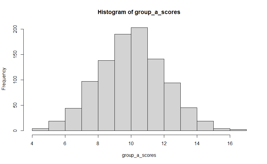
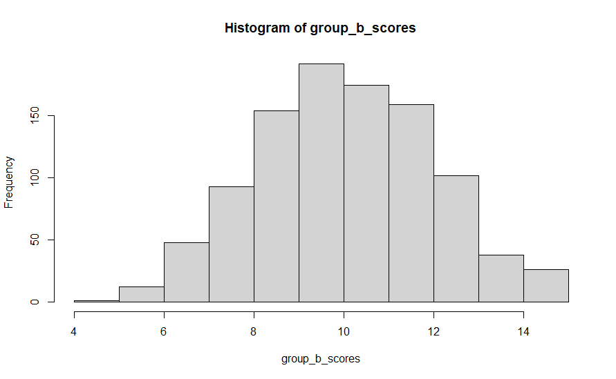
To do this, we’ll have R generate two random normal variables, corresponding to the scores of two groups A and B. Both of these will have the same properties; 1000 observations from a population designed to have a mean of 10 and a standard deviation of 2.
  group_a_scores <- rnorm(1000, mean = 10, sd = 2)
  group_b_scores <- rnorm(1000, mean = 10, sd = 2)
This is equivalent to a scenario where you’ve run an experiment with 1000 participants in your test group (A) and 1000 in your control group (B). The test intervention had no effect on the scores obtained by participants, i.e. the null hypothesis is true. But of course you would not expect the group A results to exactly match those from group B in the end because most real world outcome variables are likely to have some random variation.
We can see that in practice by checking the mean and distribution of the scores from group a and group b. In the first run I did of this code, group A’s mean was 10.03 and group B’s mean was 10.05. Close, but not exactly the same, even though they were generated from the same distribution of data. Histograms showing the distribution of scores in each case are shown below.
So now, let’s attempt to draw some statistical conclusions about whether these scores come from truly different populations – did whatever we do to group A folk lead to different outcomes that group B people obtained? The answer is of course no, but most of the time the whole point of the experiment is that we can’t know that in advance.
Imagine that in an effort to get to a conclusion faster we decided to check in on the experiment five times, at equally spaced out intervals. In this case we chose a t test as our test of significance and a threshold of p <= 0.05 as the threshold for significance.
So we’ll run a t test when we get to 200 participants in each group. If that shows significance we declare a winner. But if not then we carry on until we have 400, 600, 800 and finally the full 1000 participant results to test, at each point deciding our intervention had effect if we see see a p value of <= 0.05
In R, we can do:
t.test(group_a_scores[1:200], group_b_scores[1:200])$p.value,
to get the p value when comparing the first 200 results from group A with the first 200 results from group B.
The below script repeats this process 10000 times, each time with a newly randomly generated normal distribution for A and B.
We know that there was is no real difference between the groups, because we designed them to be the same. So anywhere we see significant differences we can consider them false positives. In the below, we calculate and store this in the false_positives variable.
number_of_trials <- 10000

significant_result_count <- 0

for (counter in seq(1, number_of_trials))
{

  # create 2 datasets that are normally distributed with the same average and standard deviations

  group_a_scores <- rnorm(1000, mean = 10, sd = 2)
  group_b_scores <- rnorm(1000, mean = 10, sd = 2)

  # Get the p values we would obtain from a t test after the first 200, 400, 600 etc. participants were available.

  p_values_for_each_check <- c(t.test(group_a_scores[1:200], group_b_scores[1:200])$p.value,
                               t.test(group_a_scores[1:400], group_b_scores[1:400])$p.value,
                               t.test(group_a_scores[1:600], group_b_scores[1:600])$p.value,
                               t.test(group_a_scores[1:800], group_b_scores[1:800])$p.value,
                               t.test(group_a_scores[1:1000], group_b_scores[1:1000])$p.value
                               )

# keep count of how many times any of those p values showed a value of <= 0.05

  significant_result_count <- significant_result_count + ifelse(min(p_values_for_each_check) <= 0.05, 1, 0)

}

# % false positive rates

false_positive_rate <- significant_result_count / number_of_trials
If checking significance early and continuing wasn’t actually a problem then we would expect a false positive rate as defined here of around 0.05, right? That was the threshold we set for our t test. But if we check what it actually was, then the first time I ran the above I got a 15% false positive rate. 14% on the second run, 15% on the third, 14% on the fourth.
You get the picture I’m sure. Instead of us incorrectly drawing the conclusion that group A is different to group B around 5% of the time, it’s about three times as likely we make that mistake. This is a big, potentially dangerous, difference! We say whatever the big fancy intervention we applied to group A members was did create a real difference in 15% of instances, even though this simulation was designed such that that cannot actually be true, and we were claiming that we had only a 5% chance of making this type of error.
Solving the too many false positives problem
So now we’re convinced that this is a real problem, what can we do about it? Assuming we do want to check on the experiment in progress multiple times, which is a perfectly sensible thing to do for the reasons discussed above, then one solution is to adjust the p value threshold you test for significance with such that the overall type 1 error rate remains at 5%, rather than performing each individual test with that same p <= 0.05 threshold.
A quick and dirty method could be to apply the equivalent of the Bonferroni correction for multiple comparison testing in general. In this case we’d divide the p value threshold for each individual test we want by the number of tests we intend to carry out. In the above example we’re planning on 5 tests, so each time we should check for a p value of 0.05/5 = 0.01.
That’s easy to do in the above script – just change the 0.05 value that’s used to calculate the significant_result_count to 0.01. I did this, and ran it a few times. The false positive rates turned out to be about 3-4% in each case (0.0356, 0.0353, 0.0342, 0.0307 etc.).
This is all fine and good from the point of view of ensuring type 1 error rates don’t exceed our specifications. In fact it gives us a slightly less than the planned 5% chance of making these errors, and hence is a conservative adjustment. But, as well as being slightly conservative, audiences may also feel peeved that the threshold for significance for each individual test is that much more stringent. If you’ve got to the point where you’ve collected all your data, then testing against a p value threshold of 0.01 as opposed to 0.05 is obviously that much harder to detect significance with. A power analysis would show that you require a larger maximum sample to detect the same effect. Sure, you may get to stop early and having tested fewer of your sample than had you been performing a conventional one-shot test. But you obviously can’t rely on that, and if you run out of the resources to test the number of participants that you maximally may need then your experiment may be doomed.
And here we’ve even ended up constructing a scenario where the overall error rate is a little lower than we required. Whilst statistically valid in terms of keeping the false positive errors to below a chosen threshold, it’s an unnecessarily inefficient approach. But honestly not a terrible one if you want a quick, dirty, slightly suboptimal but familiar solution to the problem at hand, prioritizing not declaring significance where it doesn’t exist.
Note that there’s an implicit assumption when using the Bonferroni-style adjustment method above that each of your five tests on the same data are independent from each other, which is clearly not really the case. In my second check I tested the first 400 participants against each other, half the data I was testing was in fact the same 200 participants that I’d tested in my first check. This dependence gives us an avenue to increase efficiency.
The same kind of approach can be made a little more efficient by using Pocock boundaries as opposed to the Bonferroni correction. In practice this means the p value you test for at each point can be a little higher than the Bonferroni method would suggest. According to tables such as this one from Wikipedia, for experiments such as that described above we can use a p value threshold of 0.0158 for each test, rather than 0.01. Making that adjustment to my simulation got me false positive error rates very close to the desired 5% – 0.049, 0.048, 0.054, 0.053.
One downside to even the above compensation is that you need to prespecify the number of times you intend to check on your data, and then actually follow the rule you set there. Switching from Bonferroni to Pocock boundaries does increase efficiency a little but you still need to prespecify the number of times you’re going to check in on the results, and they have to be equally spaced out.
A more flexible solution via alpha spending
So we can do better still! Assuming we count having more control and more flexibility as better – and why wouldn’t we? For this, I turned to the excellent paper by Lakens et al, “Group Sequential Designs: A Tutorial” which discusses the theory. I then turned the theory into practice by using functions from the rpact R library.
One annoyance of the methods described in the previous section is that you have to pre-specify how often you’re going to test the data and at what point. In the example I used, I was looking at the data 5 times, after collecting 20%, 40%, 60%, 80% and finally 100% of it. One approach to get around this limitation is the alpha spending approach, as documented by Lan and DeMets.
Pocock (1977), O’Brien & Fleming (1979) and Slud & Wei (1982) have proposed different methods to construct discrete sequential boundaries for clinical trials. These methods require that the total number of decision times be specified in advance. In the present paper, we propose a more flexible way to construct discrete sequential boundaries.
K. K. Gordon Lan, and David L. DeMets. “Discrete Sequential Boundaries for Clinical Trials.” Biometrika, vol. 70, no. 3
The concept here is to pre-decide on a function (“alpha spending function”) that represents the cumulative type 1 error rate throughout the experiment. At the end of the experiment, the total cumulative error rate accumulated should be the same as your desired significance level. So if you set the threshold at p <= 0.05, then the cumulative type 1 error rate of the alpha spending function must be 0.05 at the end of the experiment, no matter what it was at any individual test point during the experiment.
You’re “spending” your error as you analyse the data throughout – and as long as you don’t over-spend it (get into alpha debt?) then you won’t be inflating the false positive error rate.
The Group Sequential Designs paper mentioned above goes into a little detail about the underlying mathematics if that’s of interest.
One advantage of this approach is that, as long as you don’t decide to perform an analysis because of what you already saw in the data, you can update the alpha levels if for instance you end up analysing data at different points during the experiment than you had originally planned, or even if you ended up collecting more or less data than you had originally planned (of course the latter may still nonetheless affect the test’s power – but it won’t break the false positive error rate if you stick to this method).
You can also choose the function you want to use to spend your error by, as long as it cumulates to the right value in the end. So for example you could do a Pocock style analysis where each check uses the same significance level, or you could use any other function should you have reason to want to spend most of your error at the start of the experiment, the end of your experiment, or somewhere in between. The choice of this function will also affect your maximum required sample size, which may be the deciding factor in some cases.
How to work with alpha spending functions and analyse sequential tests in R
Now let’s look at how the practicalities of how the data analyst can use this method in the real world, in this case using the rpact R library. Much of my learning here came from browsing the many useful vignettes hosted on the rpact site.
Let’s imagine we want to plan an analysis for an experiment using the same protocol as in my simulations above. That’s to say we want to using a significance level of alpha = 0.05, and plan to check the data at a maximum of five points in time, at 20%, 40%, 60%, 80% and 100% of the data collection. I’ll also set my test power to 0.8 (i.e. beta = 0.2).
We also need to pick an alpha spending function – in this case I’ll use what rpact refers to as the asOF design, which is a function that approximates O’Brien and Fleming boundaries.
Compared to Pocock’s approach, these boundaries spend a lot less alpha towards the start of the experiment. If any detected effect isn’t significant enough to stop the experiment early, you spend increasingly more of the alpha each time you check the data as throughout the experiment. If you end up having to collect 100% of the data then the alpha for the final test is actually pretty close to the overall alpha level you wanted.
Compared to a Pocock approach, this means you have less chance of detecting statistical significance towards the start of the experiment and being able to stop early. But you have more chance of detecting a statistically significant effect at the “all-data” analysis if you didn’t see a particularly huge effect along the way, but there actually is one.
So the first thing to is set up the design of the experiment in rpact, using the getDesignGroupSequential() function. Let’s call it “my_design”.
library(rpact)

my_design <- getDesignGroupSequential(sided = 2,
                                      alpha = 0.05,
                                      beta = 0.2,
                                      informationRates = c(0.2, 0.4, 0.6, 0.8, 1),
                                      typeOfDesign = "asOF")
The first three parameters above are the concepts used in most every common frequentist hypothesis test; whether you want a one or two sided test, your type 1 error rate and your type 2 error rate.
The informationRates parameter is equivalent to the proportion of the entire planned sample you have the data for so far. So as we were going to look at 1000 participants in total, after 200, 400, 600, 800 or all of them had been processed if necessary, that’s equivalent to 0.2, 0.4, 0.6, 0,8 and 1.
The typeOfDesign is where you pick your alpha spending approach, in this case the “asOF” option as detailed above.
We can then look at a summary of the calculated design:
summary(my_design)
which shows us the cumulative amount of alpha we would spend at each stage, remembering that the final cumulative amount must equate to your chosen overall type 1 error rate, and the calculated significance scores to test against at each stage.
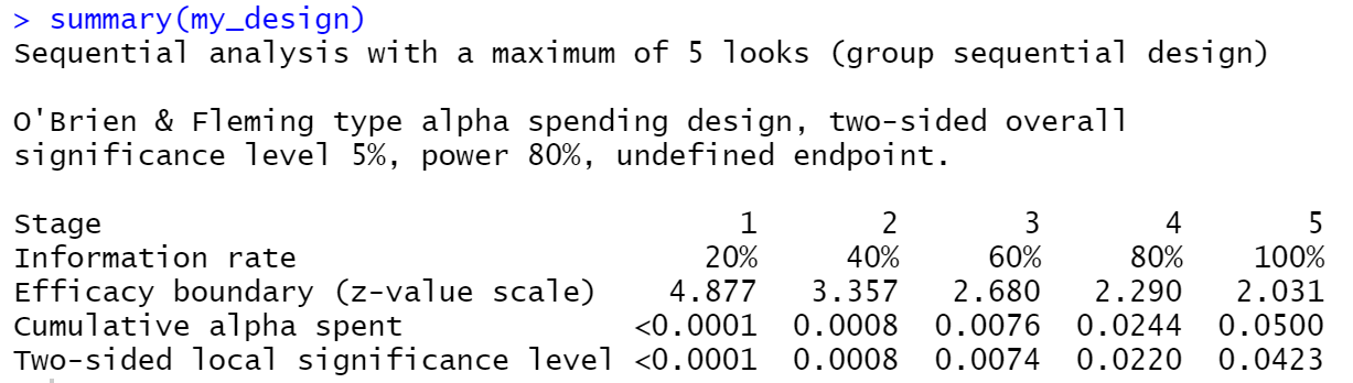
In this example you can see that because of my choice of boundaries, we are only going to see effect significance on our earlier checks if the effect is pretty dramatic. Interpret the above for instance as saying that when you perform your third check, i.e. when we collected the data for 60%, here 600, participants, use an alpha level of 0.0074 when testing for statistical significance.
Obviously, that’s a much more stringent threshold to reach than 0.05 would be. But if you did reach it, you can stop your experiment and be confident that you didn’t risk inflating the type 1 error rate.
If you do have to keep going until your last participant has been tested – which is what you would anyway have to do if you were running a “standard” non-sequential analysis – you can see that here that the relevant p value for that final test would be 0.0423. So a little less than the 0.05 you’d use in the conventional one-shot approach, but not a whole lot less. Note how this to the significance boundaries we talked about above when using the Pocock approach discussed above, which were to test against a p value of 0.0158 for every test.
A key advantage of the alpha spending approach in general is that you can safely update your design if something goes askew. Perhaps you actually don’t have the chance to run your analysis until results from 250 participants are available. You can just re-run the above getDesignGroupSequential command with informationRates of c(0.25, 0.4, 0.6, 0.8, 1) to get the appropriate boundaries to test against at each stage.
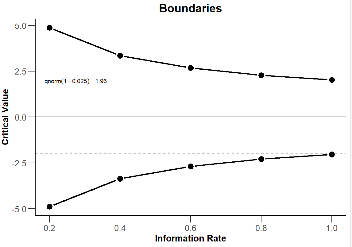
By plotting the experimental design, you can visualise how the critical value of the z score test statistic varies as you do each of the 5 checks. Recall that the critical value for a straightforward one-off test with a 95% confidence interval is 1.96.
plot(my_design, type = 1)
What about the required sample size?
Eagle-eyed observers will have noted that in my scenario so far I’ve made out that I am OK with the idea that 1000 participants per group will be a reasonable number for me to test overall. In reality, before the experiment starts, we should have carried out a sample size calculation. Here I’m going to assume that the reader has some knowledge of what and why this is and go ahead to show the functions that let us work this out for this sequential design.
Let’s assume we’re going to be testing the mean scores of the test group against those from the control group. In that case, we can feed our design from above into the function getSampleSizeMeans to see what sample size we should plan for. Per any other similar sample size calculation, we’ll need to specify the minimum effect size we want to be able to detect by the end of the analysis. This number is important for power calculations as if there are real effects of a smaller size we stand the risk of not detecting them as being statistically significant. In this case I’ll chose an effect size of 0.2, one which is traditionally considered to reflect a small effect.
my_sample_size <- getSampleSizeMeans(design = my_design,
                   groups = 2,
                   alternative = 0.2
)

summary(my_sample_size)
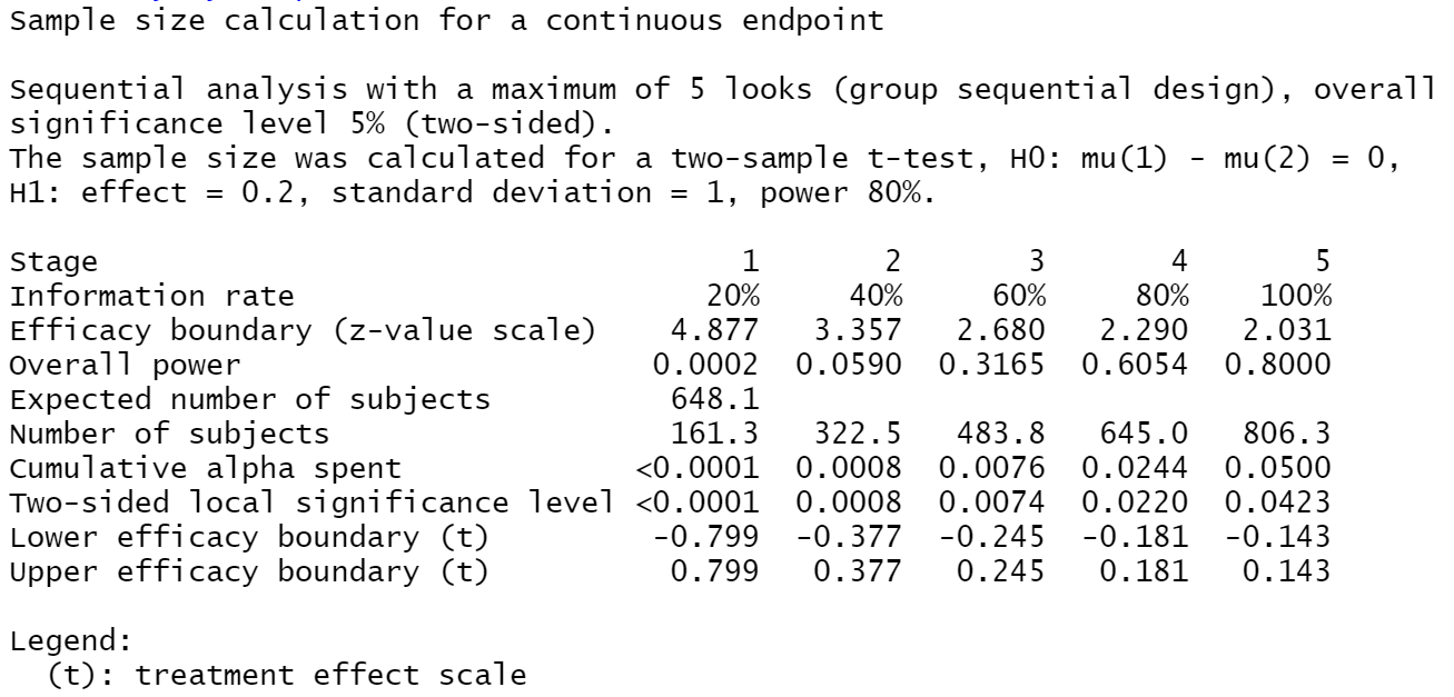
So here, looking at the ‘Number of subjects’ row we can see that if we do have to perform our full analysis, i.e. not being able to stop before the final test, then we need to have access to at least a sample of 806.3 (well, we should probably say 807!) participants to meet the alpha rate, power and effect sizes we specified above.
Compare this to a normal 1-shot test. The equivalent power calculation would be something like:
library(pwr)
pwr.t.test(d = 0.2, power = 0.8, sig.level = 0.05, type = "two.sample",  alternative = "two.sided")
which produces the result that we’d need about 787 participants to fulfill the same requirements.
Another way of thinking about this difference between a sequential design and a standard fixed design is via the “inflation factor”. That’s the increase in sample size you need to run the whole sequential design as compared to the basic one-test fixed design. You can obtain that in the output of the getDesignCharacteristics function.
getDesignCharacteristics(my_design)
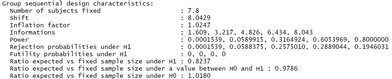
The above shows you that for this design the inflation factor is 1.0247. Thus by choosing to run our sequential design you potentially need access to 1.0247 * 787 = ~ 806 participants, which, considering rounding, is consistent with the above.
OK, so the fixed design’s requirements of 787 participants is a slightly smaller number than the 807 potentially needed for our 5-inspection sequential test. But of course at each point in our sequential test we may find significance and be able to call an end to the experiment. If we do that, then we don’t need to keep collecting sample. If that happens on our first anticipated check, then we only had to test 400 folk (200 from group A, and 200 from group B).
So, assuming we’re right about the size of the effect et al. then we can look again at the results of the summary(my_sample_size) command above to note the “Expected number of subjects”. This is calculated as, assuming there is an effect of the size we expected, the probability that we can stop at each stage multiplied by the sample we would have gathered at that particular stage. Here that is 648.1. So, if all our assumptions are right (good luck!) then on average we will only have to collect data from 649 participants; substantially fewer than for the one-off test outlined above.
However, that’s just the average rate, and only applicable if the experimental effect is at least as large as you expected, so you can never rely on being able to stop at that point. You must have a plan for collecting the whole dataset required, in this case 807 participants. But, if you ran the same experiment again and again, then the average number of participants you would need to test is 649.
Thus for a correctly specified effect, on average you’ll need fewer participants than for the conventional one-off test. But there are occasions when you’ll need a few more. Of course if there is no effect or the effect is smaller than you planned for then you will likely run through your full sample.
In any case, 807 participants is fewer participants than the 2000 I’ve been using in my example so far, so we could be confident of having enough sample to carry out this experiment if we have access to the 1000 fictional participants per group.
Carrying out the analysis once the results are in
Now let’s assume our experiment is in progress, and we’re busy collecting results. We’ve got to the point where we’ve collected the amount of sample that we wanted to for our first peek at the results. If we see significance here then we’re in a position to declare that we’ve seen an effect and hence stop the experiment. In the example experiment design I’ve been using above, this would be when you had data for 200 out of the prospective 1000 participants for each group, 400 in total. How then should we go about analysing the significance?
Well, the p value boundaries we calculated in the design summary above gave us the critical values we need, so you can go ahead and use whichever the appropriate significance test for the data and hypothesis in question would be. So if you’re wanting to compare two means from parametric-compatible data, that might be a t test, which in R is the t.test function. Recall that in practical terms all we’ve really done here is to adjust what the p value threshold to declare significance would be, so as to control the overall type 1 error rate if we do have to go ahead and check on our data several times. If you do see significance at a point using the appropriate calculated significance level then you can go home happy that you “safely” saw an effect.
If not, you keep on collecting data until you reach the next point at which you planned to check on the results. Depending on which approach to alpha spending you took this will likely involve you doing the same hypothesis test on the whole dataset so far, but at a different significance level.
You can do this testing any way you normally would, but the rpact library we’ve been using so far does have some special functions that make it easy to compute and display the output relevant to each stage of the sequential tests.
To produce the analytic results, we first need to use rpact’s getDataset function to store the results of the experiment obtained so far. For the type of “compare the mean of group A’s scores to the mean of group B’s scores” we can feed it the number of participants, the mean of the group scores and the standard deviations of the group scores for each stage.
So, for our first planned check, having reached our 200th participant in both group A and B, we know that the number of participants in each group is 200 . Using the group_a_scores and group_b_scores vector of results we generated above we can calculate the means and standard deviations of the group scores via:
group_a_mean <- mean(group_a_scores[1:200])
group_b_mean <- mean(group_b_scores[1:200])
group_a_sd <- sd(group_a_scores[1:200])
group_b_sd <- sd(group_b_scores[1:200])
For the first run I did, the mean score for group A came out as approximately 10.07 and in group B was around 9.85.
The standard deviation of scores in group A was 2.27 and in group B it was 2.09.
We can then use those summaries to create an rpact “dataset”.
test_dataset <- getDataset(n1 = 200,
                            n2 = 200,
                            means1 = group_a_mean,
                            means2 = group_b_mean,
                            stDevs1 = group_a_sd,
                            stDevs2 = group_b_sd
                            )
The documentation for getDataset shows how you can produce a dataset to compare rates or survival measures if means aren’t the appropriate measure to compare in your particular experiment.
Now we have the dataset for our first check ready, we can use the getAnalysisResults() rpact function to perform the appropriate test of significance. We need to feed into it the design of our experiment, which as part of the above code we already saved into the my_design variable. There are plenty of optional parameters for this function, but the simplest call would be:
results <- getAnalysisResults(design = my_design, dataInput = test_dataset)
If you apply the summary function to the results object you can see the status of our experiment after this first check.
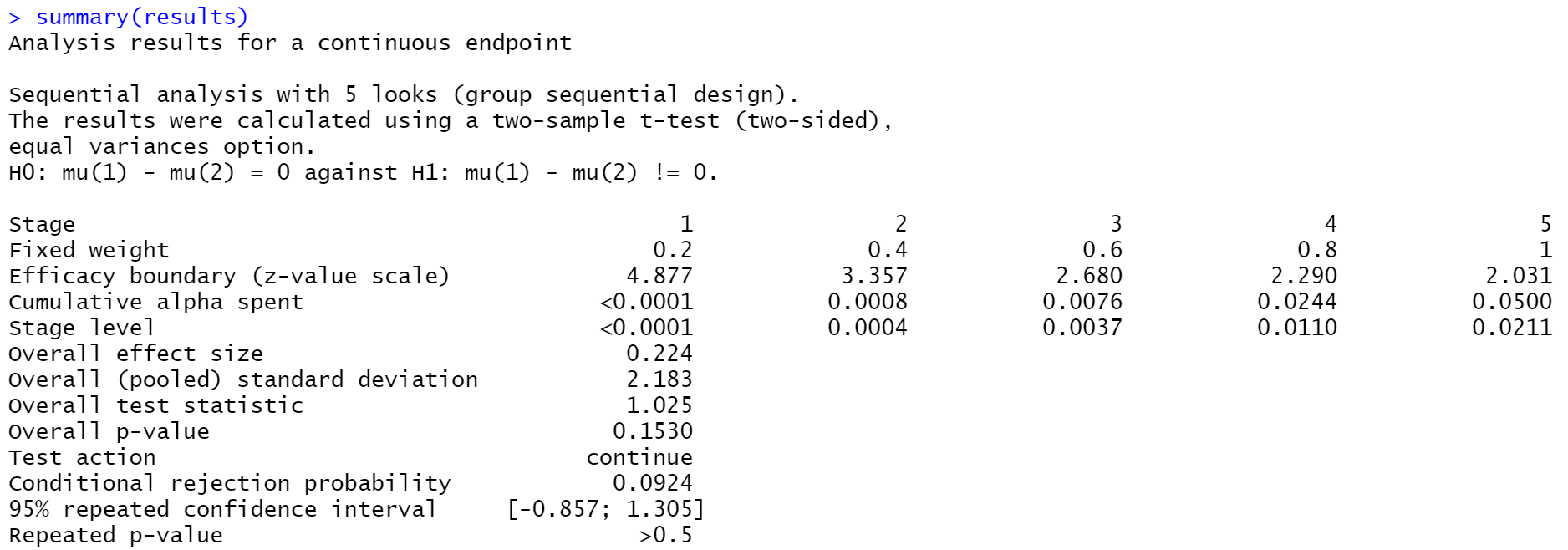
First up we get a description of our test design which we can read to double-check it matches what we want. In this case it’s spot on, using a 2 sample t-test to test a hypothesis that there’s no difference between the average of the two groups’ scores.
Next up you can see a column for each sequential test we had in our analysis plan. That was defined when we created my_design, and we’d specified 5 tests. We can see that in doing test 1 we have spent very little alpha.
What is shown as the stage level is the 1-sided p value equivalent of our two sided test – if we compare that to the results of summary(my_design) you can see it’s half of what the latter called “two-sided local significance level” for the given arm. So doubling the stage level value gives us the p value at which we would be able to conclude statistical significance at this stage from a two-sided hypothesis test. For the first check it’s <0.0001, so we’d need to have seen an extremely low p value to conclude the presence of a true difference and stop here.
As it is, we didn’t see that sort of super low p value in our data. That’s not very surprising given we know because of how we generated the data we shouldn’t expect to see any real difference between groups.
Here you can see in the “overall p-value” row that the p value we did actually see in this, our first check, was 0.1530. Per the rpact step-by-step tutorial vignette that’s again a one-sided version, unadjusted. If we were to calculate the two sided p value for this data via e.g. t.test we’d see a p value of double that, i.e. 0.3059 in this case. Note that this is the case in the output of this particular rpact function even if the final analysis is being run for a two-sided test.
We’ll see later the library produce the results for the two-sided test which it calls the “final p value”. However, that’s not available yet as, having not seen statistically significant differences between groups at this stage, we must carry on collecting data until we have enough sample to perform our second planned check. Here that means 400 participants per group. We know this as the “Test action” shown in the results summary above says “continue”. So continue we must.
Another potentially interesting output of the results summary about is the 95% repeated confidence interval row. Here we can see that the confidence interval for the differences between group A and group B score is from -0.857 to 1.305. A difference of 0 is thus very much within those bounds, reinforcing the fact we haven’t detected a significant difference between these groups.
There are various rpact functions to pull out specific parts of the results. These may be useful if you want to process these values in a later part of your analysis. For example, if you want to extract the confidence interval mentioned in the previous paragraph you can use the getRepeatedConfidenceIntervals() function.
getRepeatedConfidenceIntervals(design = my_design, dataInput = my_dataset, stage = 1)
`

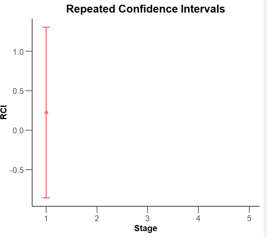
There are also various interesting plots that can be automatically made from this and other rpact outputs. If you wish to plot the above confidence interval, you can plot the results of the call to getAnalysisResults() specifying a plot type of 2.
plot(results, type = 2)
So, moving on, let’s fast forward to what the analysis results look like once the experiment has been run to the end. Recall that this means either we detected significance in one of our interim looks, or we got to the end of the planned experiment (in this case having tested 1000 participants from each group) and failed to detect the statistically significant difference we specified as enough for us to reject the null hypothesis.
As a sneak preview of the results of this run of my test sample, let it be known that, as expected, none of the checks produced evidence of a real difference between group A and group B results. In this case we know that’s the correct conclusion.
So to produce the final result for this analysis, first create the dataset, feeding in vectors to represent the results seen in each of our five checks.
test_dataset <- getDataset(
  n1 = c(200, 200, 200, 200, 200),
  n2 = c(200, 200, 200, 200, 200),
  means1 = c(10.074046, 9.765305, 10.045700, 9.935283, 9.993715),
  means2 = c(9.850319, 9.996358, 10.079409, 10.024584, 10.005320),
  stDevs1 = c(2.268386, 2.051473, 1.908592, 2.045020, 2.113241),
  stDevs2 = c(2.093249, 2.221950, 1.958057, 1.895951, 1.808735)
)
Note that we’re passing in the sample size, means and standard deviations from the relevant cohort of each of group A and B (or 1 and 2 as this function’s parameters call them).
So the second entry in the means1 vector, 9.765305, is the mean of the scores from participants numbers 201-400, i.e. the “new” sample collected after our first check that will form part of our second check. It’s not the cumulative mean of all participants 1-400.
In reality, I would personally calculate the means and standard deviations dynamically in the code, but here for clarity I’ve written them out as fixed numbers.
Next, get the analysis results, in the same way as before, and display the summary.
results <- getAnalysisResults(design = my_design, dataInput = test_dataset)

summary(results)
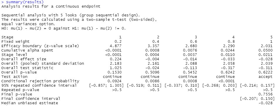
Looking at column 5, the final check we did, we can see that the “Cumulative alpha spent” is now 0.05. That’s the overall p value threshold we specified we wanted to perform our analysis at.
The test action row shows we had to continue each time after our first four checks as we hadn’t detected the appropriate level of significance to reject the null hypothesis and declare an effect. On the final check the action is “accept”, as we now have to accept the null hypothesis of no difference between groups, having now finished our planned experiment.
From the “Final p-value” row, we see that the p value reached at the end of the experiment, this time for the two-sided test that we’d specified, is 0.7556. This is substantially above 0.05 hence we can’t reject the null hypothesis. The final confidence interval also very much surrounds zero, reinforcing that verdict.
We can visualise the evolution of the confidence intervals through the checks by performing that type 2 plot again.
plot(results, type = 2)
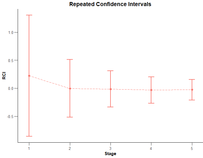
As would normally be the case, you can see how the range of the confidence intervals tends to shrink as we get to later stages and narrow in on a more precise idea of any effect seen due to having the benefit of a larger amount of our sample.
If you’re wanting direct access to the final p value then there’s a getFinalPValue() function for exactly that.
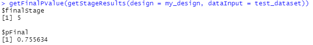
In fact the function that we fed into getFinalPValue, getStageResults() gives us some useful information per stage by itself. If we pass it the design and result data it’ll tell us all sorts of things about the situation at each of our 5 checks.

Many of those datapoints were already shown to us when we looked at the summary of the getAnalysisResults() output, but the means, standard deviations and sample sizes per stage might be of use.
Let’s see what the results look like in the case that we do detect a significant difference between our two groups. For this I’ll set up a couple of datasets that we know are different from each other based on their definition. We’ll generate some random normal data again, but this time such that group A has a higher mean score than group B.
group_a_scores <- rnorm(1000, mean = 12, sd = 2)
group_b_scores <- rnorm(1000, mean = 10, sd = 2)
We can then run through the exact same procedure featured above. For brevity, I’ll just be showing the summary() of the call to getAnalysisResults() below. To be specific, this would be the result after our first check, where we had collected 200 participants from both groups.
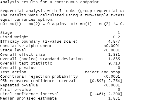
Note specifically the “Test action” now reads “reject and stop”, as opposed to before when it read “continue”. This is because, if we look at the final p value, we’ve already reached a point where the difference between group scores appears to be highly statistically significant – of course the p value isn’t exactly 0, but it’s so low that the software has rounded it down to such. The 95% confidence interval of the difference shows us that at this point it’s between 1.46 and 2.20 – which is appropriate enough given we know the actual difference is 2 given how we constructed the data.
Thus we can reject the null hypothesis at this first check, and stop the experiment without having to go ahead and collect data from the rest of the 2000 total participants – whilst remaining confident that what we saw is a real effect. Or at least that the risk of the effect being a false positive is what we decided up front we could live with (p <= 0.05) and not something with a secretly much inflated risk of this kind of error due to us planning to check in on the experiment multiple times.
Using simulation to check controlling the type 1 error worked
To be fair, given we exposed the risk of type 1 error inflation of taking multiple peeks without controlling for that at the start of this article by a process of simulation, we should do the same again using this spending alpha approach to make sure it does actually solve the problem I’m claiming it does!
We’ll use the same set up as we started off with near the start, constructing two datasets we know were generated from the same distribution. Hence the “correct” conclusion is that they are not significantly different from each other. Again we’ll simulate checking in 5 times during the experiment, stopping if we detect a statistically significant difference at any point. We’ll again do this 10000 times and see how often we get what we know is effective a false positive result. When we did this above, specifying an alpha of 0.05 for our hypothesis tests but without controlling for the fact we were peeking at the data potentially up to 5 times we found that instead of a 5% type 1 error rate we actually ended up with one about 3 times higher, in the region of 15%. Bad news indeed.
So let’s give it a whirl with the alpha spending method outlined above.
number_of_trials <- 10000

significant_result_count <- 0

for (counter in seq(1, number_of_trials))
{
  group_a_scores <- rnorm(1000, mean = 10, sd = 2)
  group_b_scores <- rnorm(1000, mean = 10, sd = 2)


  my_dataset <- getDataset(
    n1 = c(200, 200, 200, 200, 200),
    n2 = c(200, 200, 200, 200, 200),
    means1 = c(mean(group_a_scores[1:200]), mean(group_a_scores[201:400]), mean(group_a_scores[401:600]), mean(group_a_scores[601:800]), mean(group_a_scores[801:1000])),
    means2 = c(mean(group_b_scores[1:200]), mean(group_b_scores[201:400]), mean(group_b_scores[401:600]), mean(group_b_scores[601:800]), mean(group_b_scores[801:1000])),
    stDevs1 = c(sd(group_a_scores[1:200]), sd(group_a_scores[201:400]), sd(group_a_scores[401:600]), sd(group_a_scores[601:800]), sd(group_a_scores[801:1000])),
    stDevs2 = c(sd(group_b_scores[1:200]), sd(group_b_scores[201:400]), sd(group_b_scores[401:600]), sd(group_b_scores[601:800]), sd(group_b_scores[801:1000]))
  )

  significant_result_count <- significant_result_count + ifelse(getFinalPValue(design = my_design, dataInput = my_dataset, stageResults = getStageResults(my_design, my_dataset, stage = 5))$pFinal <= 0.05, 1, 0)
}

# % false positive

significant_result_count / number_of_trials
The first time I ran the above I got a false positive rate of 0.052, the second was 0.045 and the third ended up as 0.051.
These are all very near to 0.05, and thus I feel reassured that this method does successfully keep the type 1 error rate at the level we had originally specified, whilst enabling us to peek at the experiment several times before it’s complete.
